ggplot(mpg, aes(x = displ)) + geom_histogram()10 Position scales and axes
You are reading the work-in-progress third edition of the ggplot2 book. This chapter should be readable but is currently undergoing final polishing.
Position scales are used to control the locations of visual entities in a plot, and how those locations are mapped to data values. Every plot has two position scales, corresponding to the x and y aesthetics. In most cases this is clear in the plot specification, because the user explicitly specifies the variables mapped to x and y explicitly. However, this is not always the case. Consider this plot specification:
In this example the y aesthetic is not specified by the user. Rather, the aesthetic is mapped to a computed variable: geom_histogram() computes a count variable that gets mapped to the y aesthetic. The default behaviour of geom_histogram() is equivalent to the following:
ggplot(mpg, aes(x = displ, y = after_stat(count))) + geom_histogram()Because position scales are used in every plot, it is useful to understand how they work and how they can be modified. In this chapter we’ll discuss this in detail. The chapter is organised into four main sections:
- Section 10.1 discusses continuous position scales. In addition to covering core topics like controlling scale limits (Section 10.1.1), breaks (Section 10.1.4), and labels (Section 10.1.6), there are sections providing a detailed coverage of scale transformations (Section 10.1.7) as well as the subtle issues that arise when you need to zoom in or zoom out on a plot (Section 10.1.2 and Section 10.1.3).
- Section 10.2 discusses date/time scales, a special type of continuous scale. Because dates and times are a little more complicated than a standard continuous variable, ggplot2 provides special scales to help you control the major and minor breaks (Section 10.2.1 and Section 10.2.2) and the labels (Section 10.2.3) for date/time data.
- Section 10.3 discusses discrete position scales. It covers limits, breaks, and labels in Section 10.3.1 and axis label customisation in Section 10.3.2.
- Section 10.4 discusses binned position scales.
10.1 Numeric position scales
The most common continuous position scales are the default scale_x_continuous() and scale_y_continuous() functions. In the simplest case they map linearly from the data value to a location on the plot. There are several other position scales for continuous variables—scale_x_log10(), scale_x_reverse(), etc—most of which are convenience functions used to provide easy access to common transformations, discussed in in Section 10.1.7.
10.1.1 Limits
All scales have limits that specify the values of the aesthetic over which the scale is defined. It’s very natural to think about these limits for numeric position scales, as they map directly to the ranges of the axes. By default, the limits are calculated from the range of the data variable, but sometimes you will need to set the limits manually using the limits argument to the scale function. Whenever the scale is continuous, as is the case for numeric position scales, this should be a numeric vector of length two. If you only want to set the upper or lower limit, you can set the other value to NA.
Manually setting scale limits is a common task when you need to ensure that scales in different plots are consistent with one another. To illustrate why this is necessary consider this faceted plot:
ggplot(mpg, aes(displ, hwy)) +
  geom_point() +
  facet_wrap(vars(year))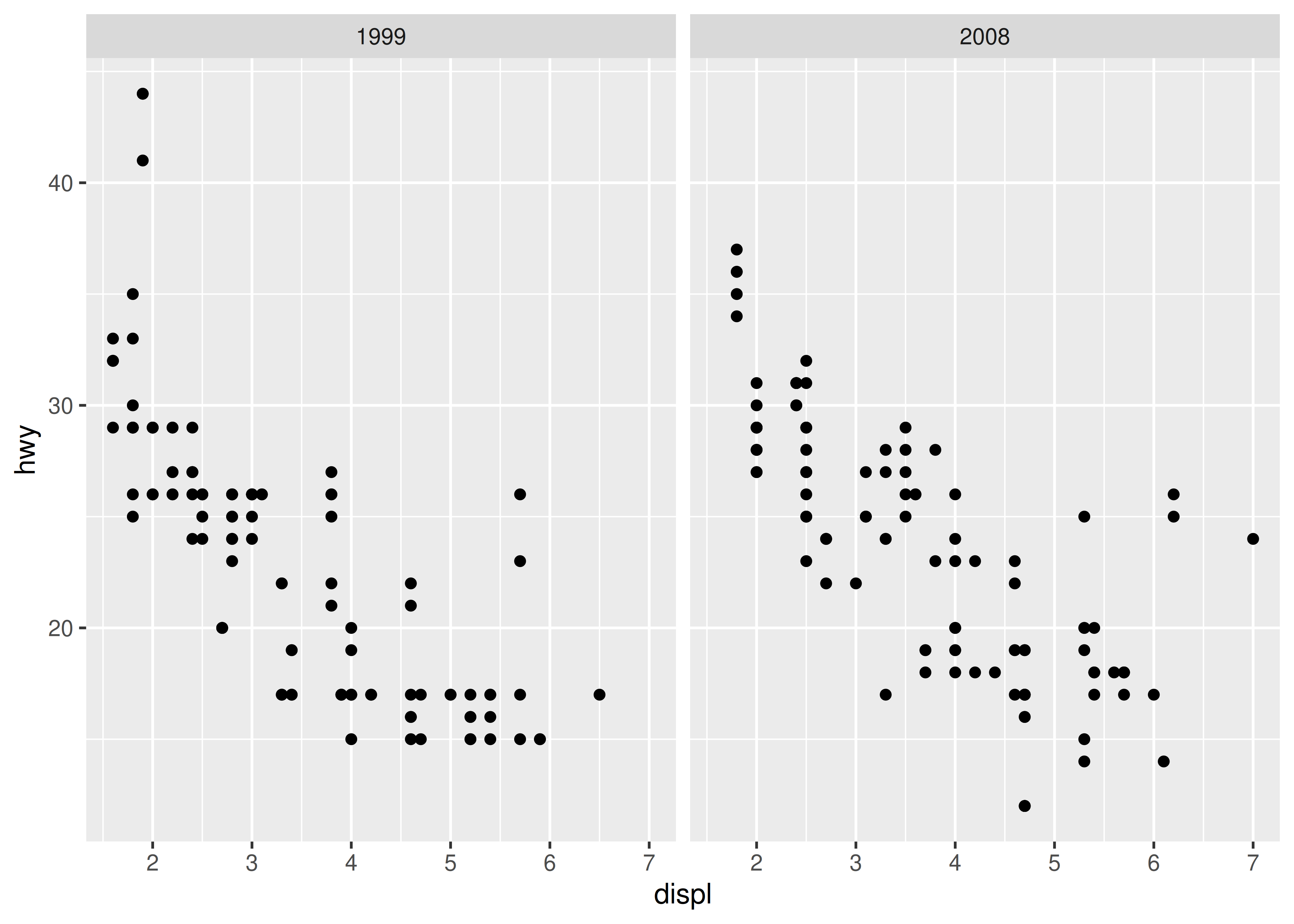
In this plot, ggplot2 has automatically ensured that both facets have the same axis limits, making visual comparison of the two scatter plots easy. However, when creating the plots individually the scale limits in different plots will often be inconsistent:
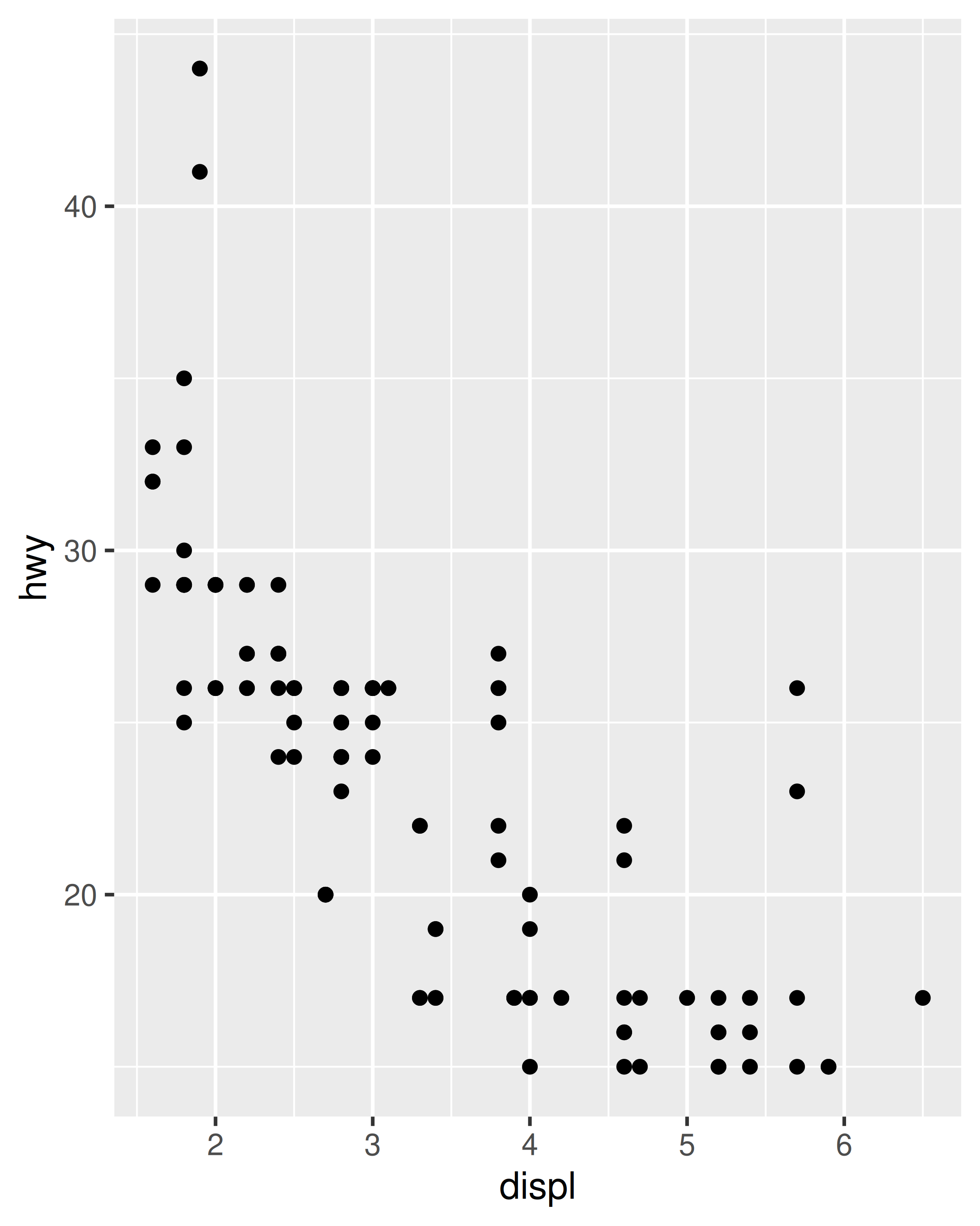
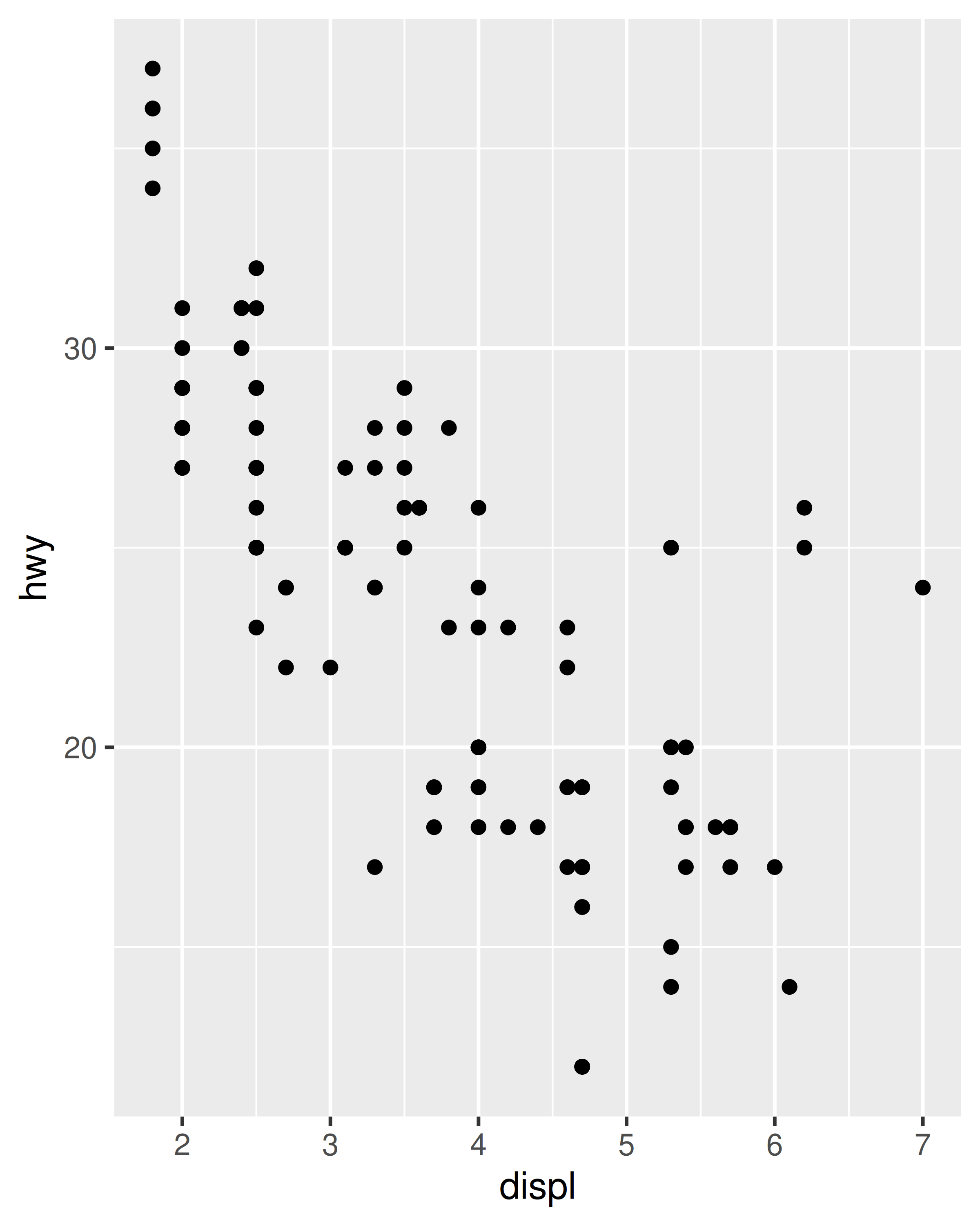
Each plot makes sense on its own, but visual comparison between the two is difficult due to the inconsistent axis scaling. To ensure consistent axis scaling, we can set the limits argument to each scale separately:


However, this code is a little unwieldy. Because modifying scale limits is such a common task, ggplot2 provides the lims() convenience function to simplify the code. Analogous to the labs() function used to specify axis labels (Section 8.1), lims() takes name-value pairs as inputs: the argument name is used to specify the aesthetic, and the value is used to specify the scale limits.
In the special case where only one axis limit needs to be specified, ggplot2 also provides xlim() and ylim() helper functions, which can save you a few keystrokes. In practice lims() tends to be more useful, because it can be used to set limits for several aesthetics at once. You’ll see an example of lims() applied to non-position aesthetics in Section 11.3.5.
10.1.2 Zooming in
The examples in the previous section expand the scale limits beyond the range spanned by the data. It is also possible to narrow the default scale limits, but care is required: when you truncate the scale limits, some data points will fall outside the boundaries you set, and ggplot2 has to make a decision about what to do with these data points. The default behaviour in ggplot2 is to convert any data values outside the scale limits to NA. This means that changing the limits of a scale is not always the same as visually zooming in to a region of the plot. If your goal is to zoom in on part of the plot, it is usually better to use the xlim and ylim arguments of coord_cartesian():
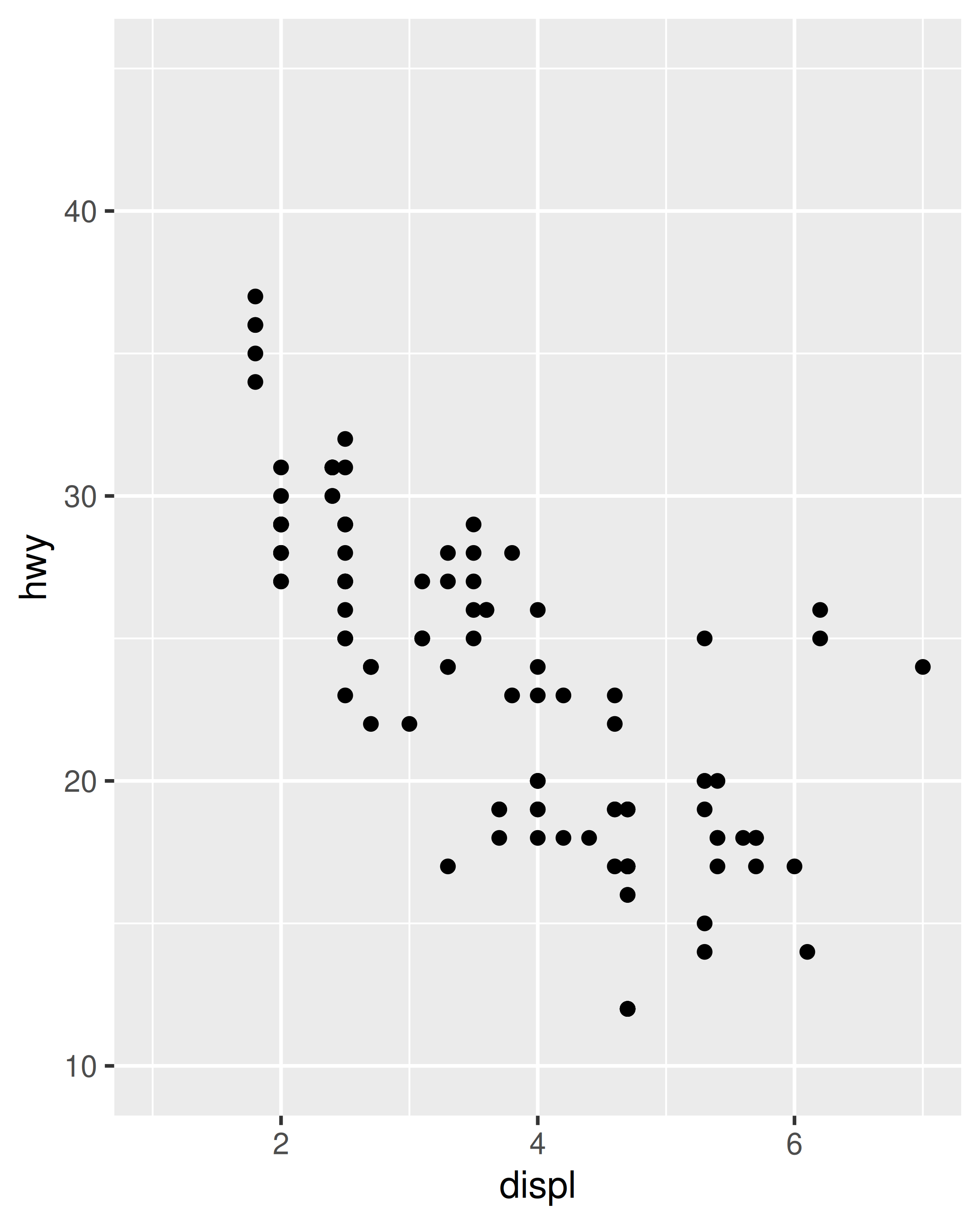
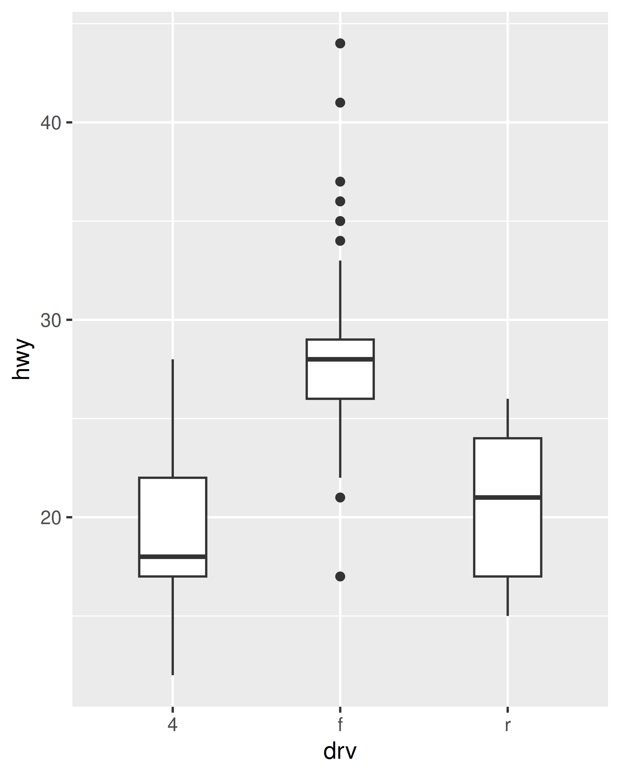
base <- ggplot(mpg, aes(drv, hwy)) +
  geom_hline(yintercept = 28, colour = "red") +
  geom_boxplot()

base
base + coord_cartesian(ylim = c(10, 35)) # works as expected
base + ylim(10, 35) # distorts the boxplot
#> Warning: Removed 6 rows containing non-finite outside the scale range
#> (`stat_boxplot()`).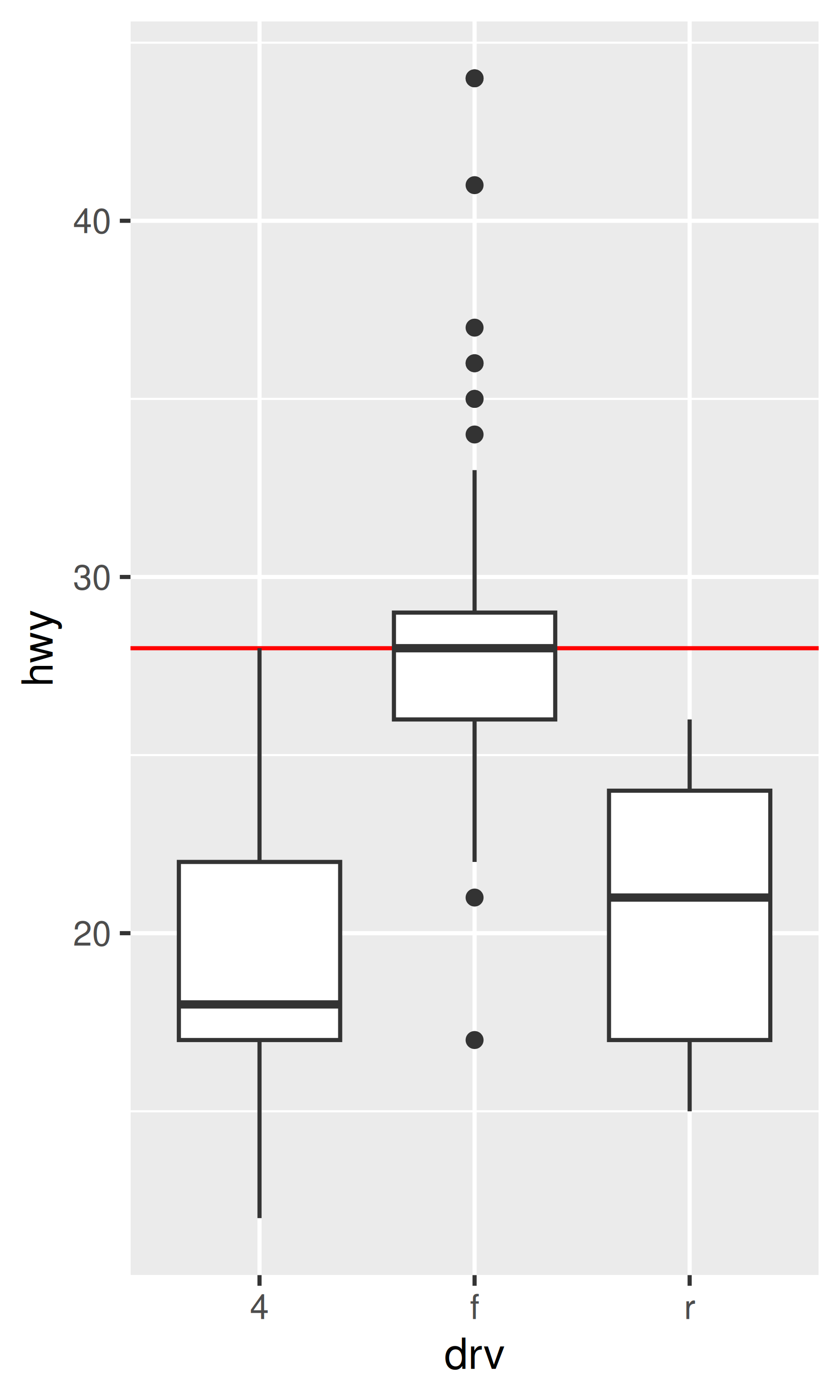
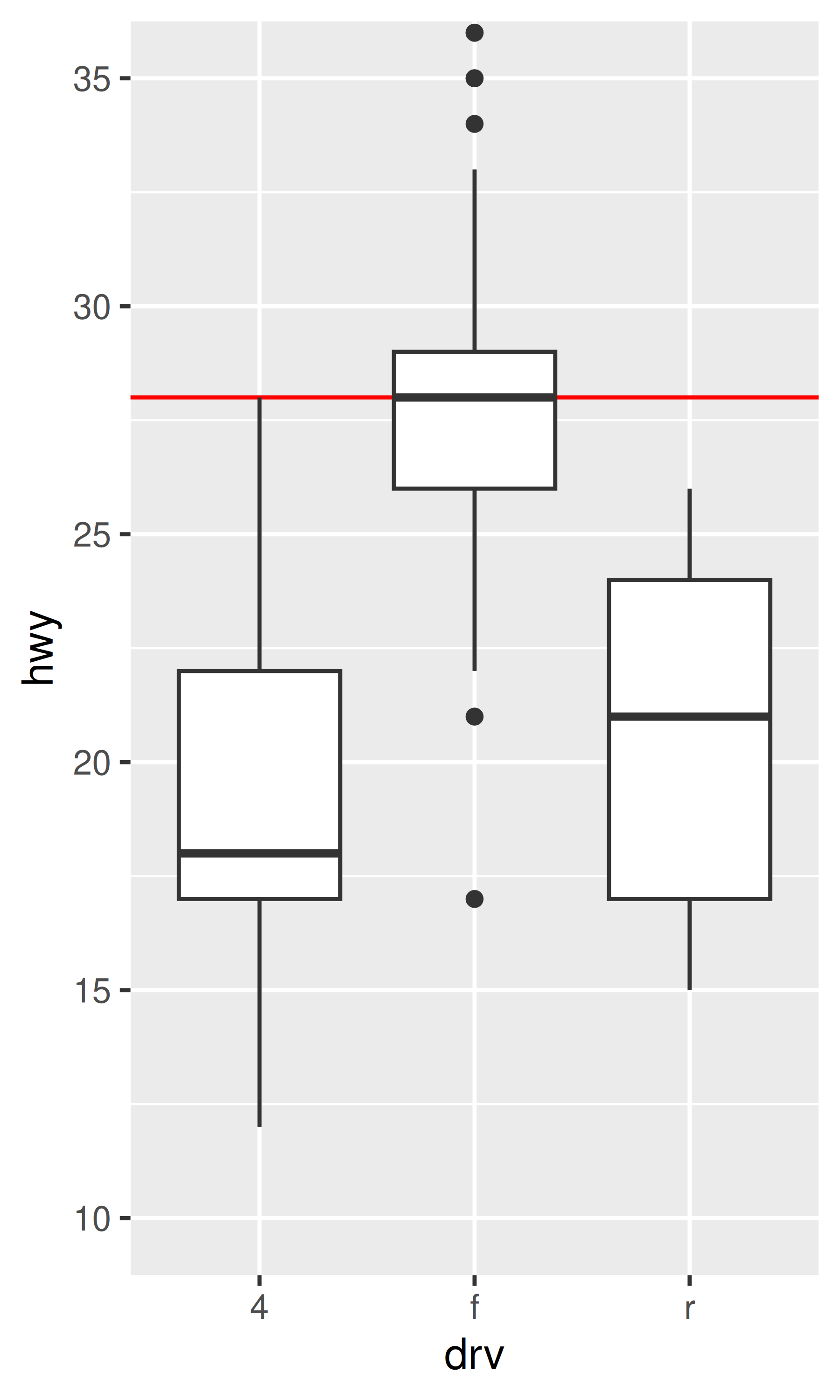
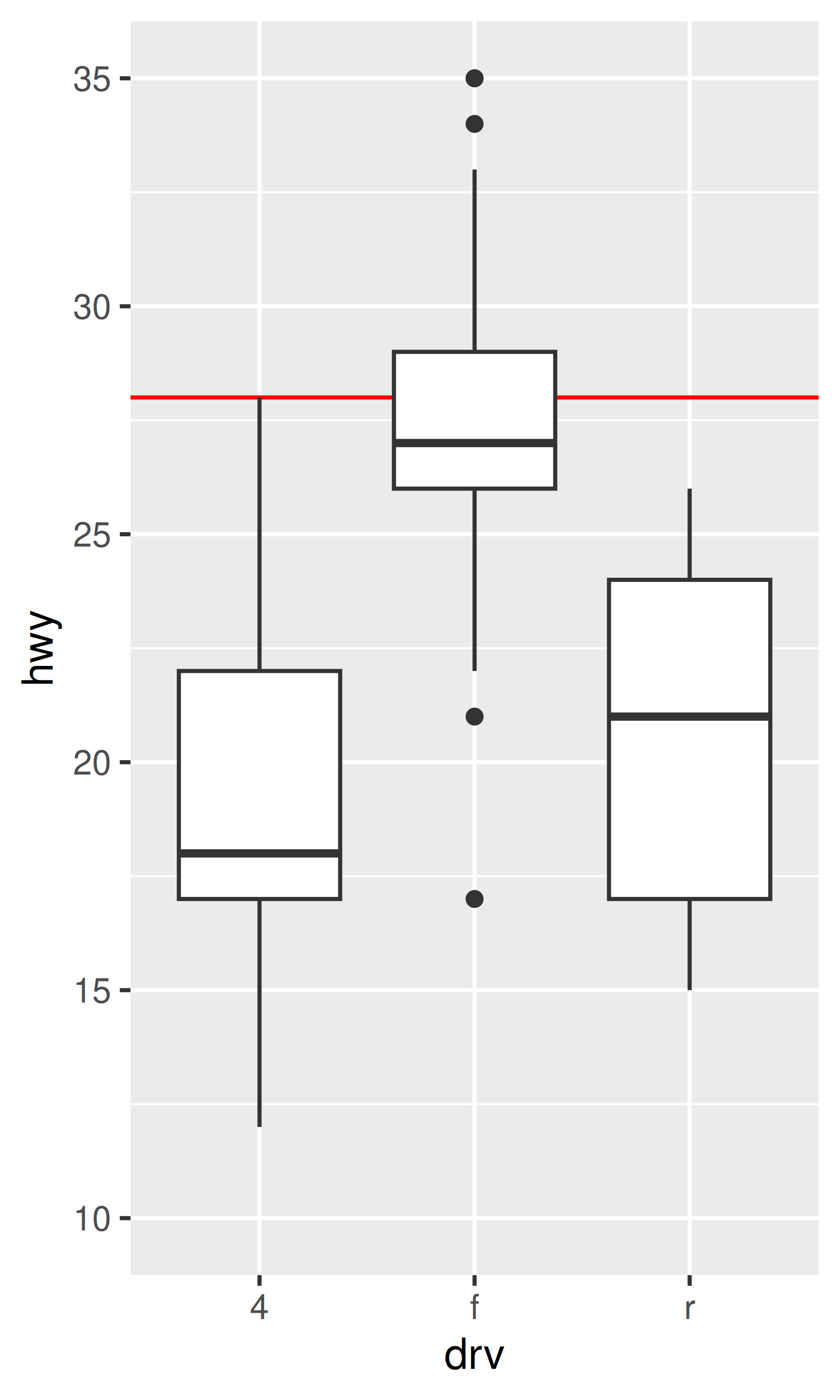
The only difference between the left and middle plots is that the latter is zoomed in. Some of the outlier points are not shown due to the restriction of the range, but the boxplots themselves remain identical. In contrast, in the plot on the right one of the boxplots has changed. When modifying the scale limits, all observations with highway mileage greater than 35 are converted to NA before the stat (in this case the boxplot) is computed. Because these “out of bounds” values are no longer available, the end result is that the sample median is shifted downward, which is almost never desirable behaviour. With the benefit of hindsight it’s clear this wasn’t a good design choice, because it is a common source of confusion for users. Unfortunately, it would be very hard to change this default without breaking a lot of existing code.
You can learn more about coordinate systems in Section 15.1. To learn more about how “out of bounds” values are handled for continuous and binned scales, see Section 14.4.
10.1.3 Visual range expansion
If you have eagle eyes, you’ll have noticed that the visual range of the axes actually extends a little bit past the numeric limits that we have specified in the various examples. This ensures that the data does not overlap the axes, which is usually (but not always) desirable. You can override the defaults setting the expand argument, which expects a numeric vector created by expansion().
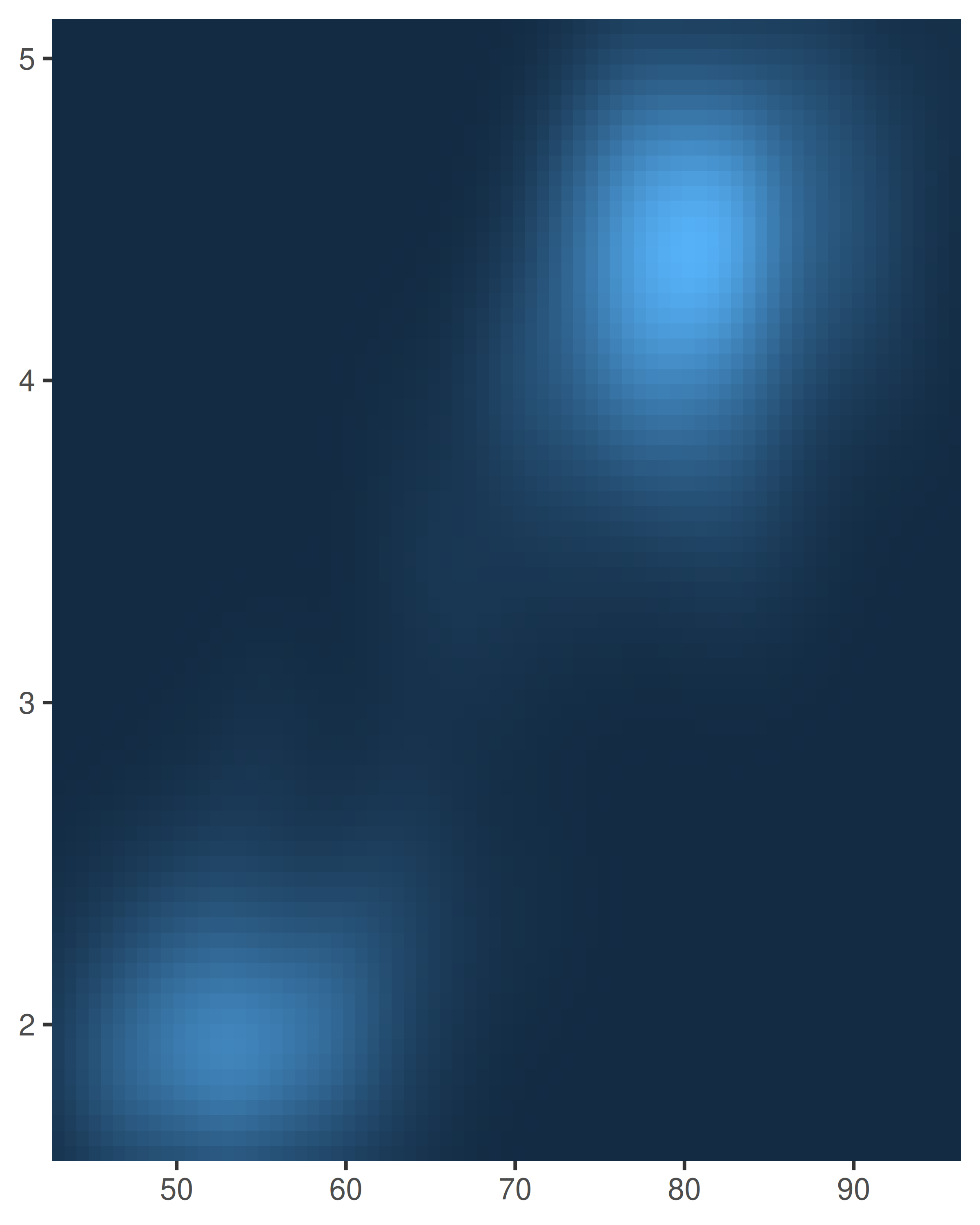
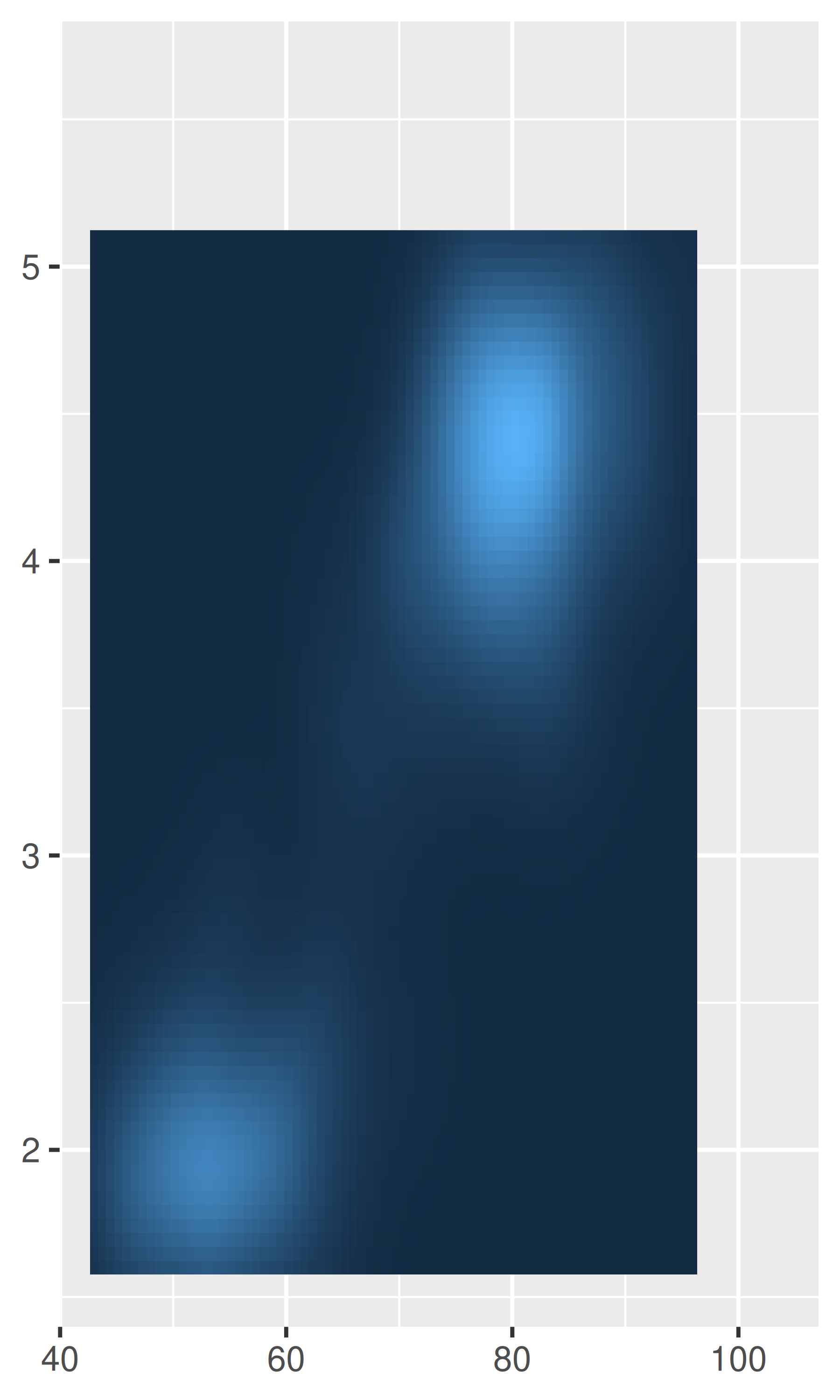
For example, one case where it’s usually preferable to remove this space is when using geom_raster(), which we can achieve by setting expand = expansion(0):
base <- ggplot(faithfuld, aes(waiting, eruptions)) +
  geom_raster(aes(fill = density)) +
  theme(legend.position = "none") +
  labs(x = NULL, y = NULL)

base
base +
  scale_x_continuous(expand = expansion(0)) +
scale_y_continuous(expand = expansion(0)) 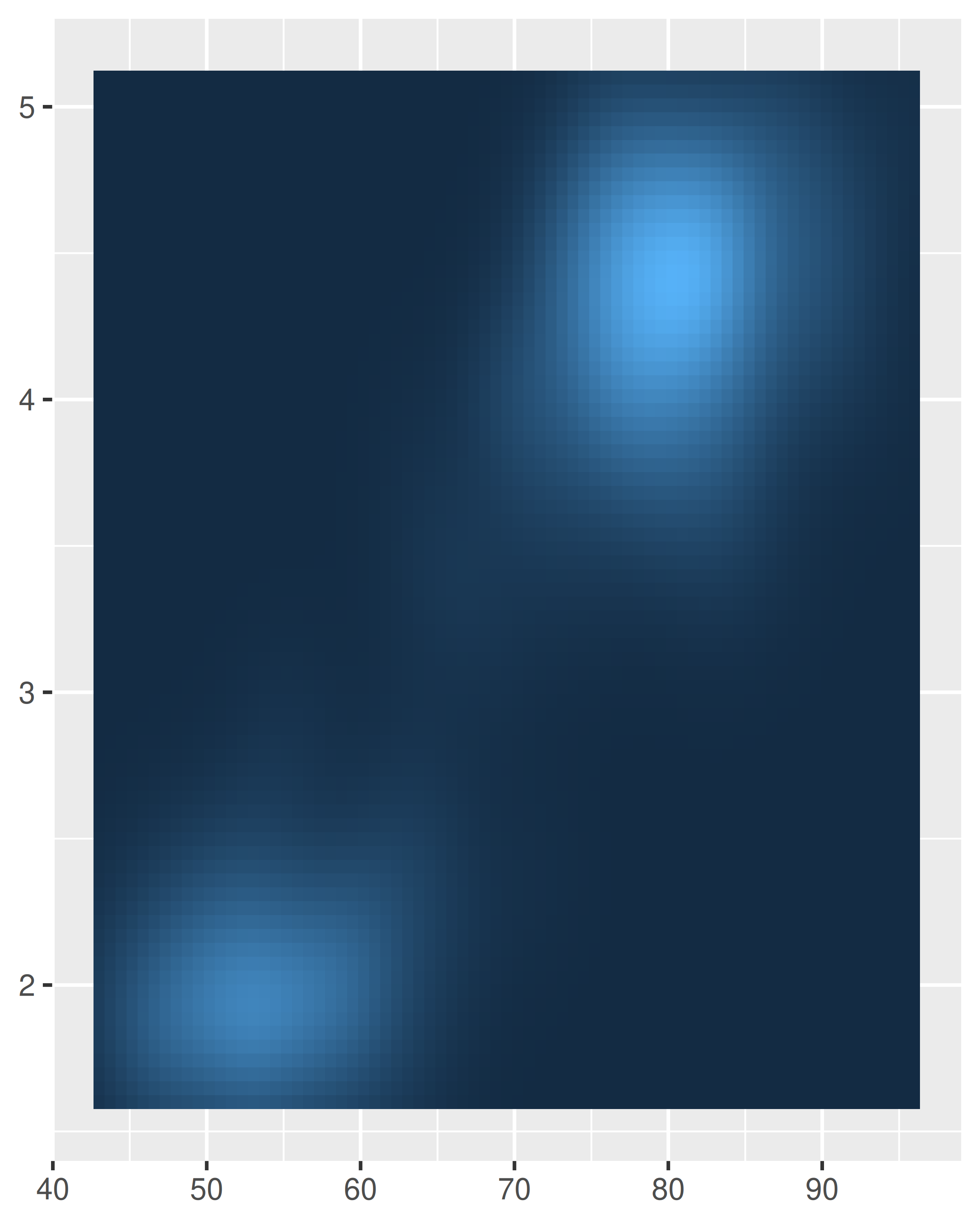
Axis expansions are described in terms of an “additive” factor, which specifies a constant space added to outside of the nominal axis limits, and a “multiplicative” one that adds space defined as a proportion of the size of the axis limit. These correspond to the add and mult arguments to expansion(), which can be length one (if the expansion is the same on both sides) or length two (to set different expansions on each side):
# Additive expansion of three units on both axes
base +
  scale_x_continuous(expand = expansion(add = 3)) +
  scale_y_continuous(expand = expansion(add = 3))

# Multiplicative expansion of 20% on both axes
base +
  scale_x_continuous(expand = expansion(mult = .2)) +
  scale_y_continuous(expand = expansion(mult = .2))

# Multiplicative expansion of 5% at the lower end of each axes,
# and 20% at the upper end; for the y-axis the expansion is
# set directly instead of using expansion()
base +
  scale_x_continuous(expand = expansion(mult = c(.05, .2))) +
  scale_y_continuous(expand = c(.05, 0, .2, 0))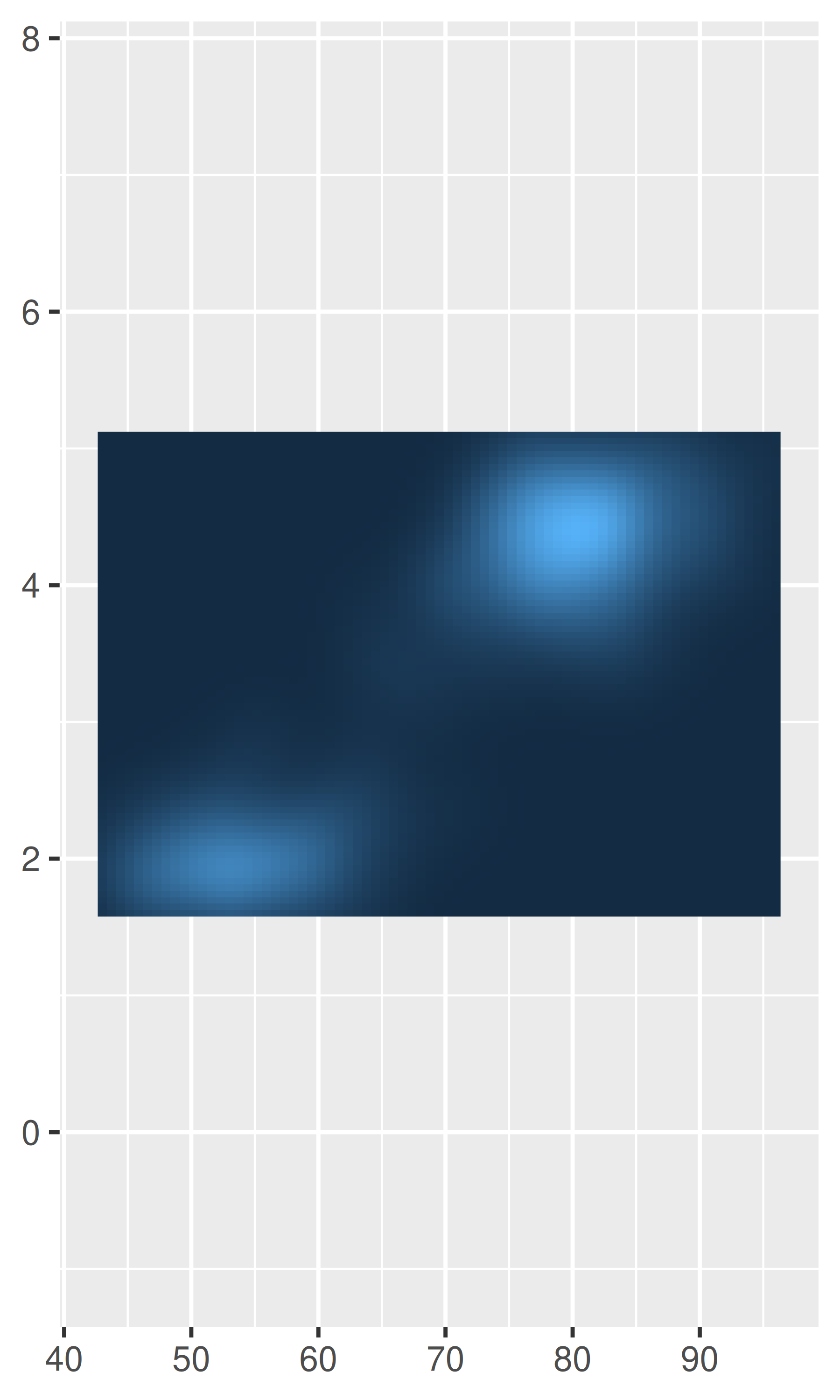
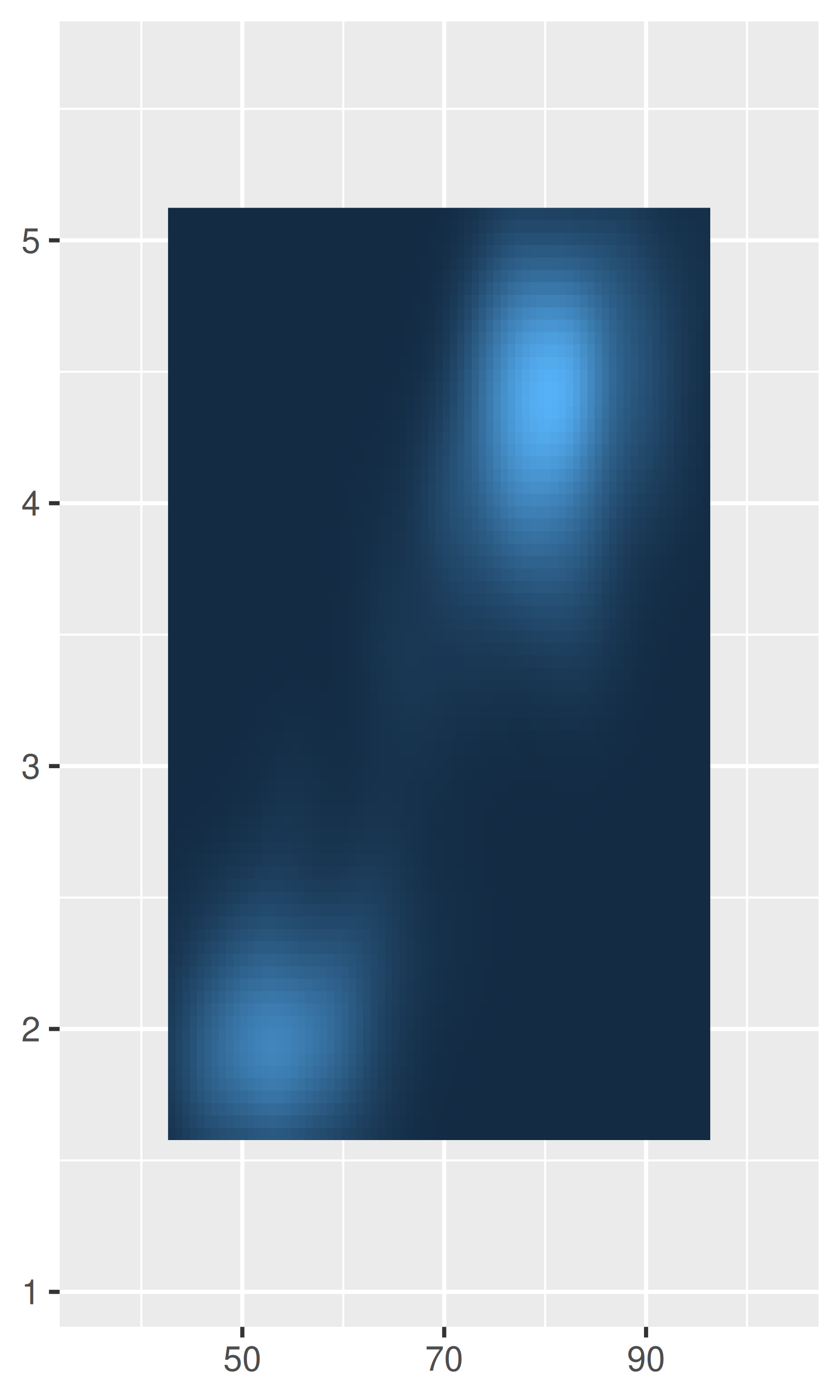
Note the different behaviour in the left and middle plots: the add argument is specified on the same scale as the data variable, whereas the mult argument is specified relative to the axis range.
10.1.4 Breaks
Setting the locations of the axis tick marks is a common data visualisation task. In ggplot2, axis tick marks and legend tick marks are both special cases of “scale breaks”, and can be modified using the breaks argument to the scale function. We’ll illustrate this using a toy data set that will reappear in several places throughout this part of the book:
toy <- data.frame(
  const = 1,
  up = 1:4,
  txt = letters[1:4],
  big = (1:4)*1000,
  log = c(2, 5, 10, 2000)
)
toy
#>   const up txt  big  log
#> 1     1  1   a 1000    2
#> 2     1  2   b 2000    5
#> 3     1  3   c 3000   10
#> 4     1  4   d 4000 2000
To set breaks manually, pass a vector of data values to breaks, or set breaks = NULL to remove the breaks and the corresponding tick marks entirely. In the plot below, removing the y-axis breaks also removes the corresponding grid lines:
base <- ggplot(toy, aes(big, const)) +
  geom_point() +
  labs(x = NULL, y = NULL) +
  scale_y_continuous(breaks = NULL)

base
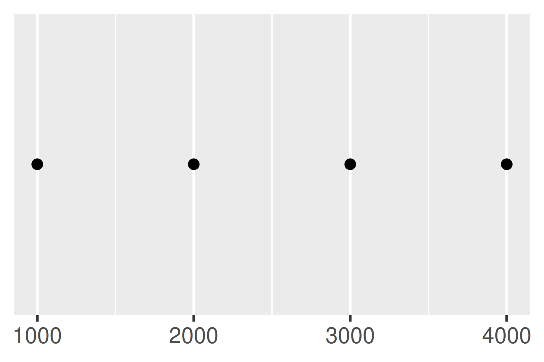
Alternatively, notice that when the breaks are set manually it moves the major gridlines and the minor gridlines between them:
It is also possible to pass a function to breaks. This function should have one argument that specifies the limits of the scale (a numeric vector of length two), and it should return a numeric vector of breaks. You can write your own break function, but in many cases there is no need, thanks to the scales package (Wickham and Seidel 2020). It provides several tools that are useful for this purpose:
-
scales::breaks_extended()creates automatic breaks for numeric axes. -
scales::breaks_log()creates breaks appropriate for log axes. -
scales::breaks_pretty()creates “pretty” breaks for date/times. -
scales::breaks_width()creates equally spaced breaks.
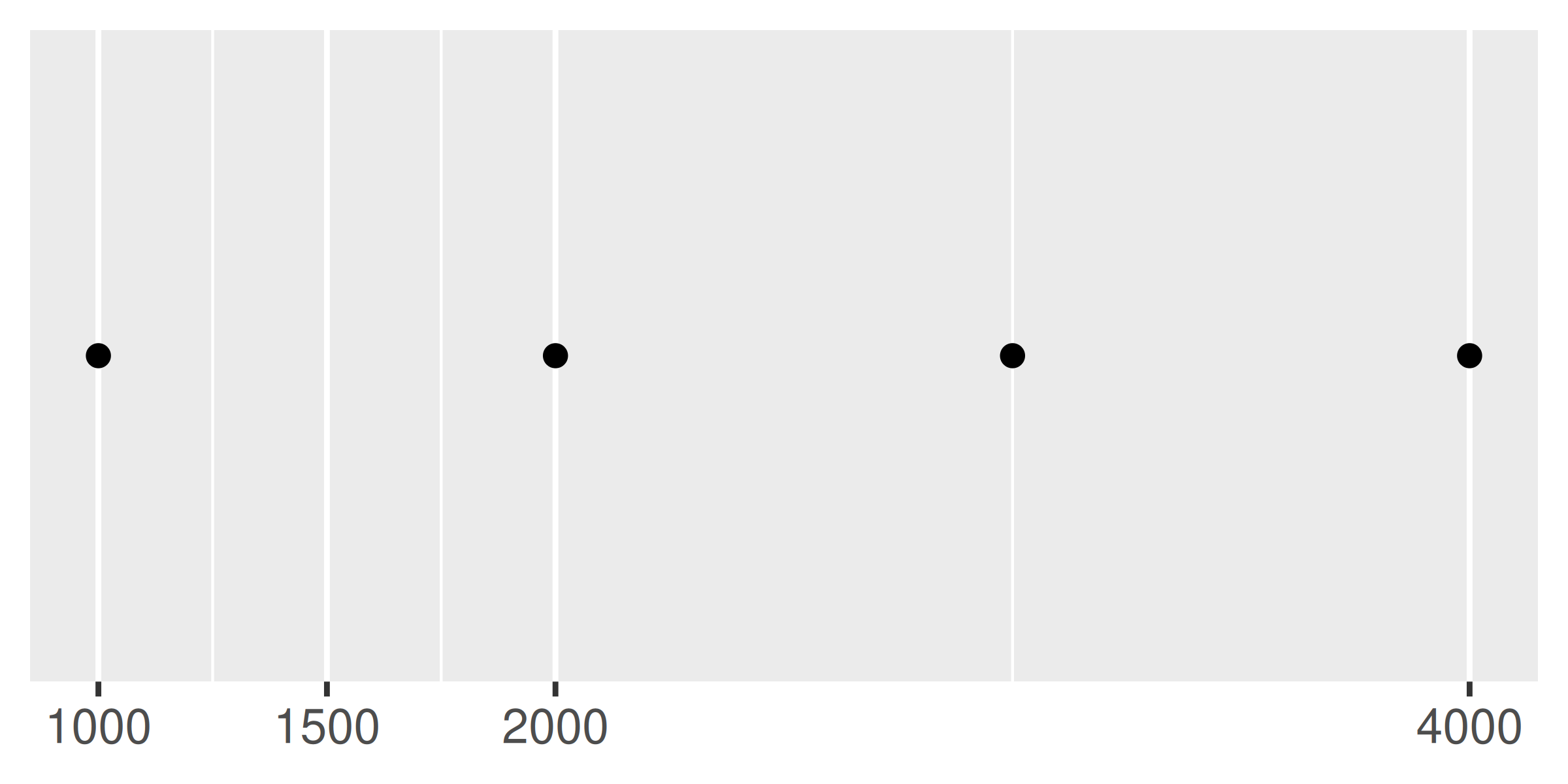
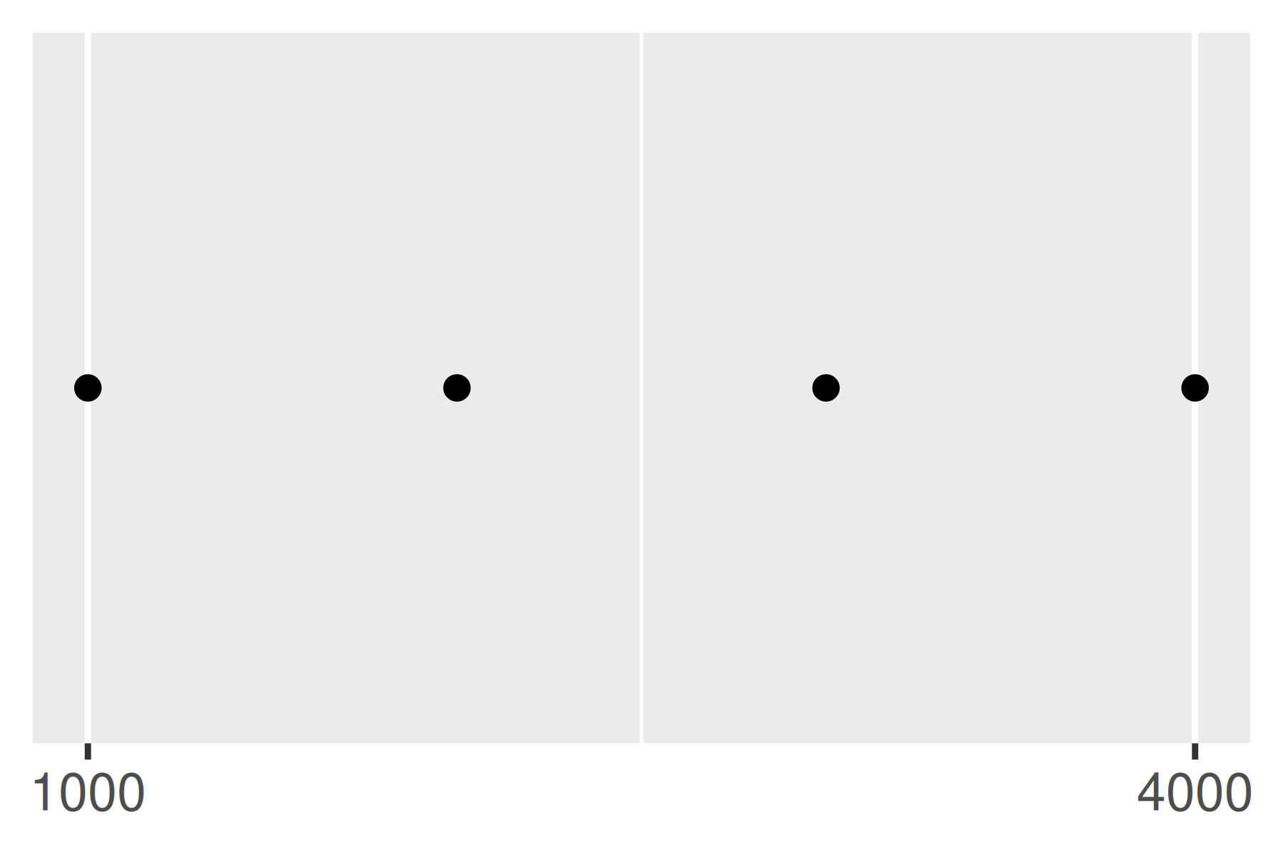
The breaks_extended() function is the standard method used in ggplot2, and accordingly the first two plots below are the same. We can alter the desired number of breaks by setting n = 2, as illustrated in the third plot. Note that breaks_extended() treats n as a suggestion rather than a strict constraint. If you need to specify exact breaks it is better to do so manually.
base
base + scale_x_continuous(breaks = scales::breaks_extended())
base + scale_x_continuous(breaks = scales::breaks_extended(n = 2))
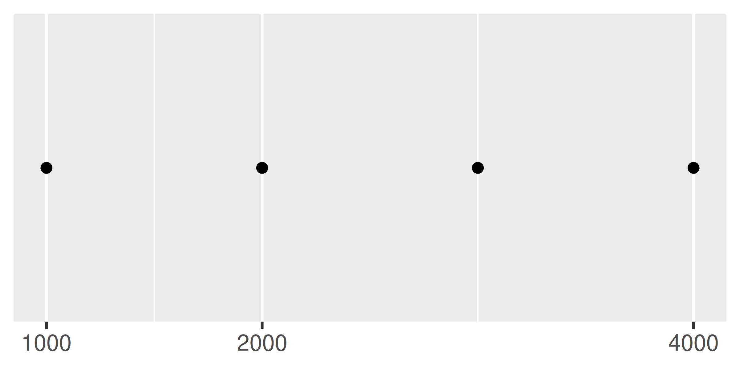
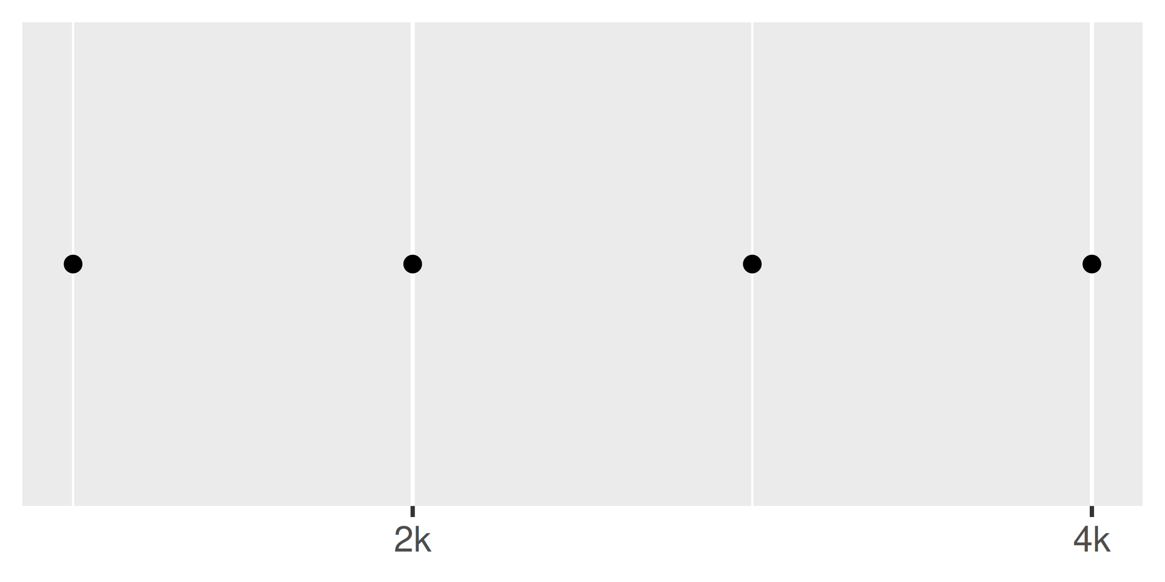
Another approach that is sometimes useful is specifying a fixed width that defines the spacing between breaks. The breaks_width() function is used for this. The first example below shows how to fix the width at a specific value; the second example illustrates the use of the offset argument that shifts all the breaks by a specified amount:
base +
  scale_x_continuous(breaks = scales::breaks_width(800))
base +
  scale_x_continuous(breaks = scales::breaks_width(800, offset = 200))
base +
  scale_x_continuous(breaks = scales::breaks_width(800, offset = -200))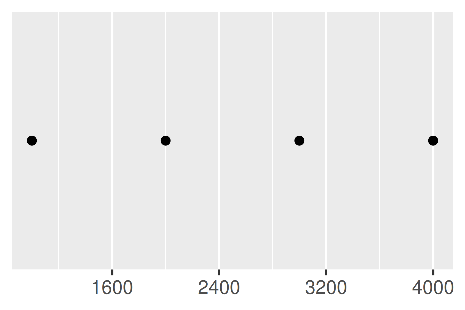
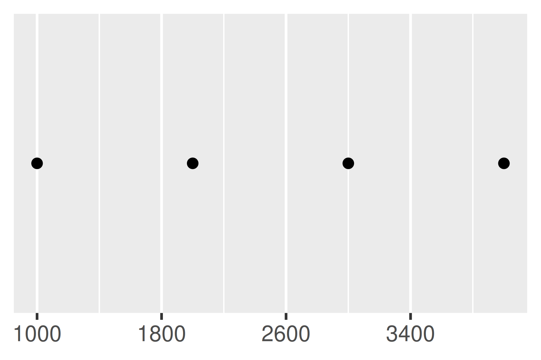
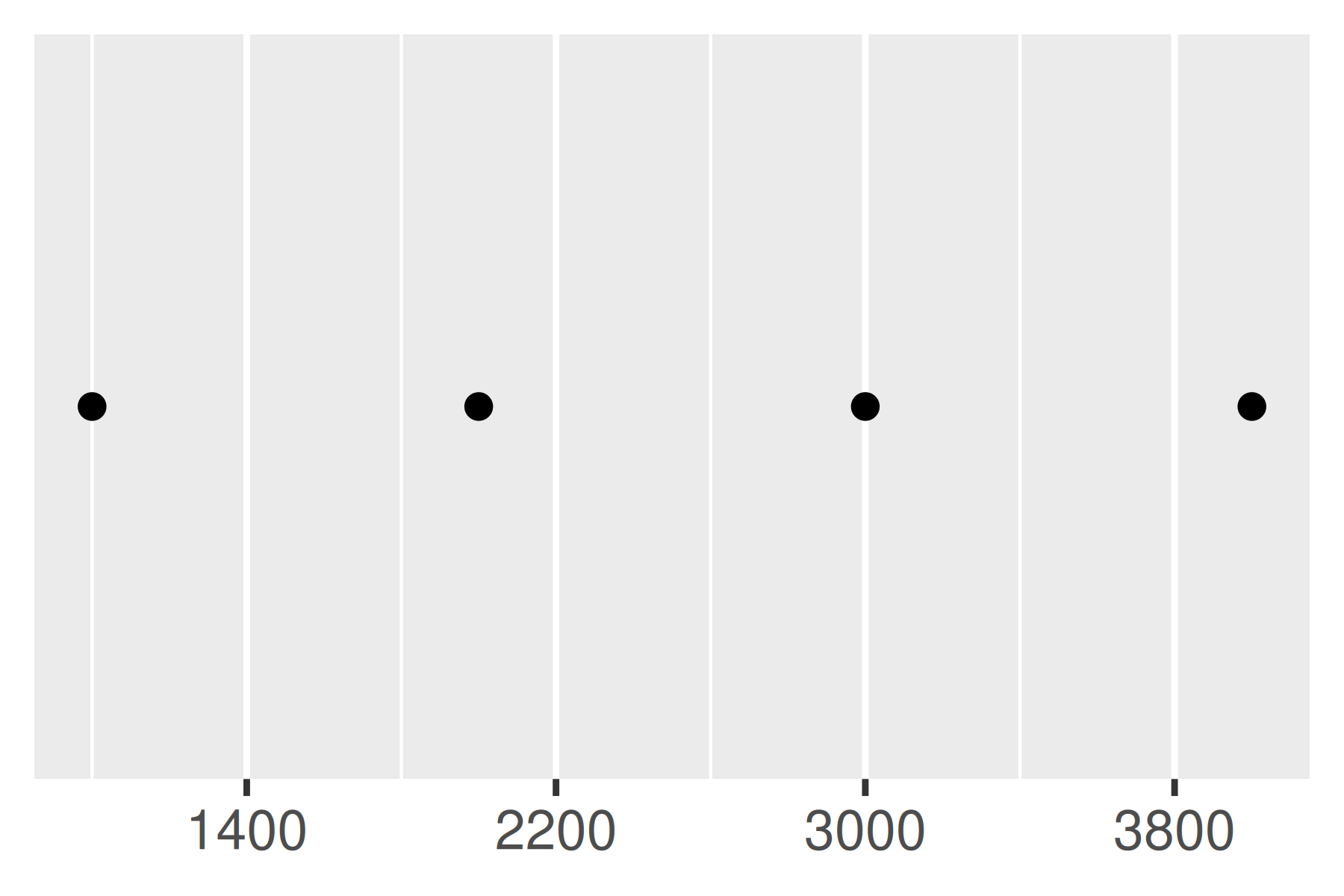
Notice the difference between setting an offset of 200 and -200.
10.1.5 Minor breaks
You can adjust the minor breaks (the unlabelled faint grid lines that appear between the major grid lines) by supplying a numeric vector of positions to the minor_breaks argument.
Minor breaks are particularly useful for log scales because they give a clear visual indicator that the scale is non-linear. To show them off, we’ll first create a vector of minor break values (on the transformed scale), using %o% to quickly generate a multiplication table and as.numeric() to flatten the table to a vector.
mb <- unique(as.numeric(1:10 %o% 10 ^ (0:3)))
mb
#>  [1]     1     2     3     4     5     6     7     8     9    10    20    30
#> [13]    40    50    60    70    80    90   100   200   300   400   500   600
#> [25]   700   800   900  1000  2000  3000  4000  5000  6000  7000  8000  9000
#> [37] 10000
The following plots illustrate the effect of setting the minor breaks:
base <- ggplot(toy, aes(log, const)) +
  geom_point() +
  labs(x = NULL, y = NULL) +
  scale_y_continuous(breaks = NULL)

base + scale_x_log10()
base + scale_x_log10(minor_breaks = mb)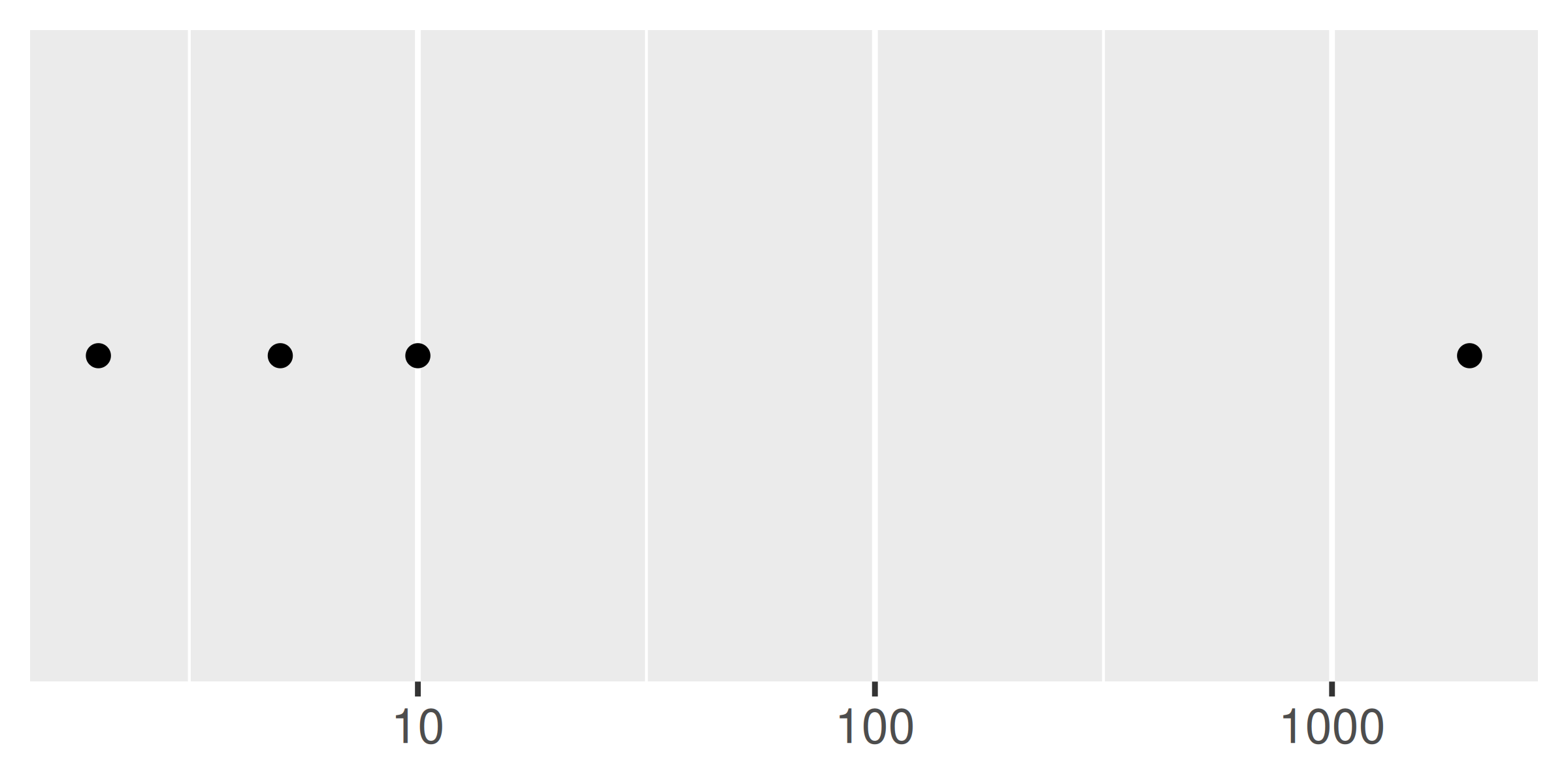
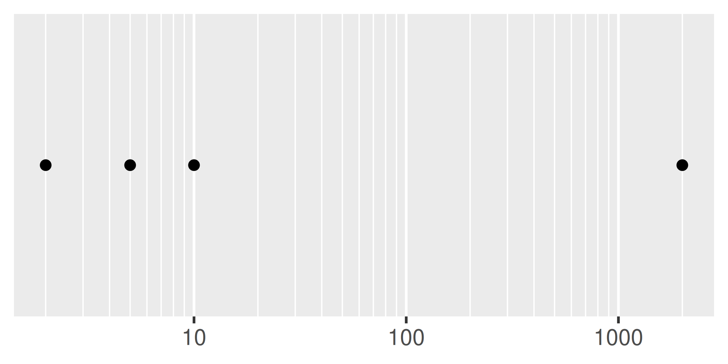
As with breaks, you can also supply a function to minor_breaks, such as scales::minor_breaks_n() or scales::minor_breaks_width() functions that can be helpful in controlling the minor breaks.
10.1.6 Labels
Every break is associated with a label and these can be changed by setting the labels argument to the scale function:

Often you don’t need to set the labels manually, and can instead specify a labelling function in the same way you can for breaks. A function passed to labels should accept a numeric vector of breaks as input and return a character vector of labels (the same length as the input). Again, the scales package provides a number of tools that will automatically construct label functions for you. Some of the more useful examples for numeric data include:
-
scales::label_bytes()formats numbers as kilobytes, megabytes etc. -
scales::label_comma()formats numbers as decimals with commas added. -
scales::label_dollar()formats numbers as currency. -
scales::label_ordinal()formats numbers in rank order: 1st, 2nd, 3rd etc. -
scales::label_percent()formats numbers as percentages. -
scales::label_pvalue()formats numbers as p-values: <.05, <.01, .34, etc.
A few examples are shown below to illustrate how these functions are used:
base <- ggplot(toy, aes(big, const)) +
geom_point() +
labs(x = NULL, y = NULL) +
scale_x_continuous(breaks = NULL)
base
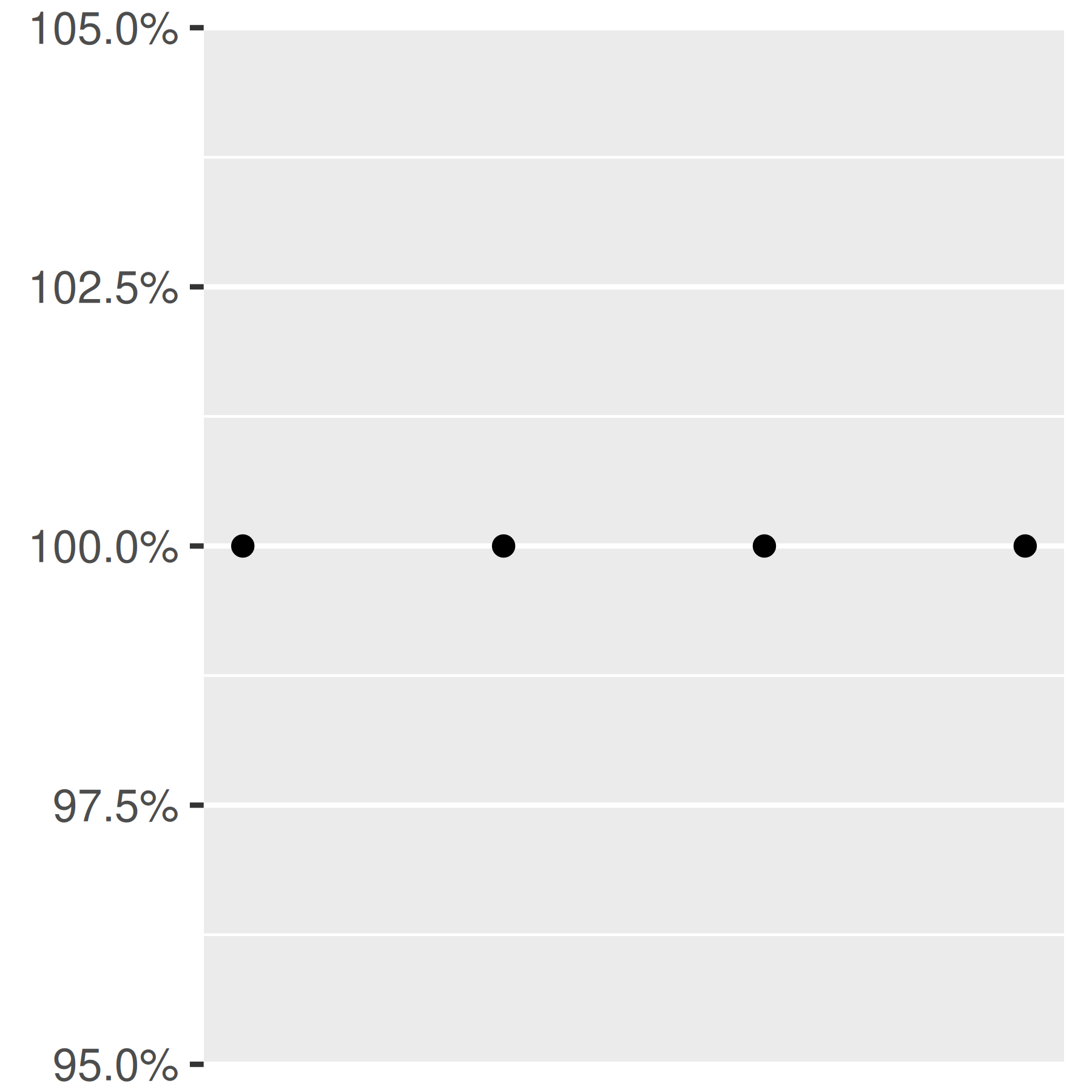
base + scale_y_continuous(labels = scales::label_percent())
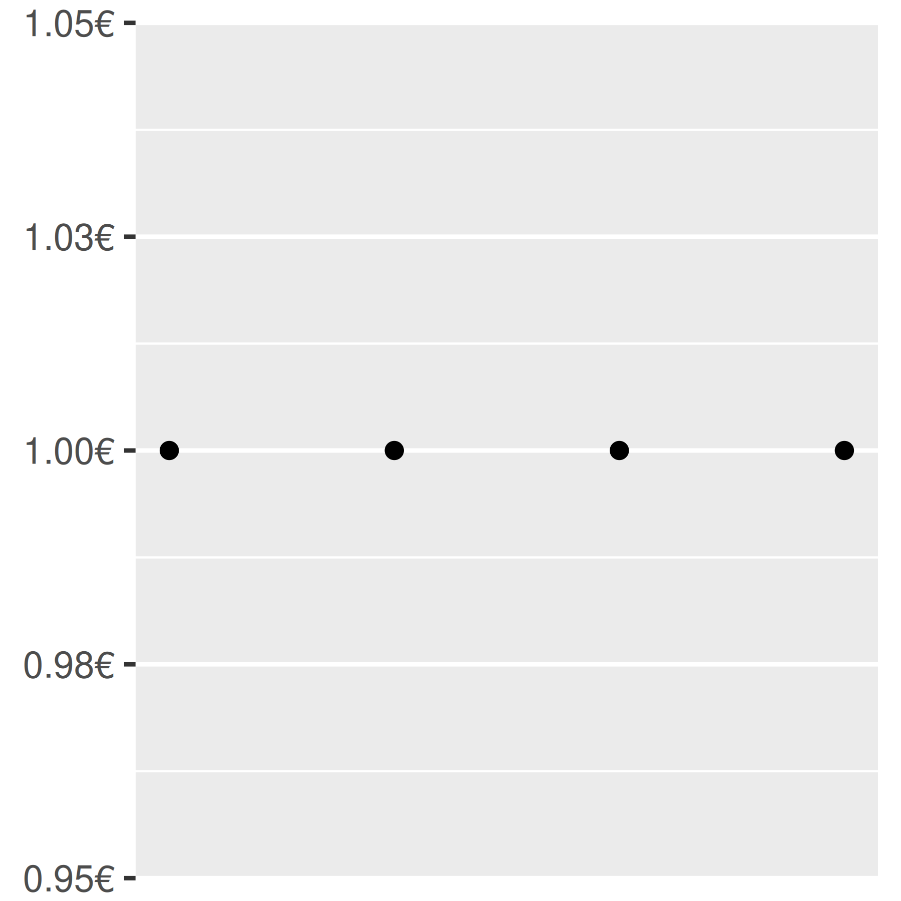
base + scale_y_continuous(
labels = scales::label_dollar(prefix = "", suffix = "€")
)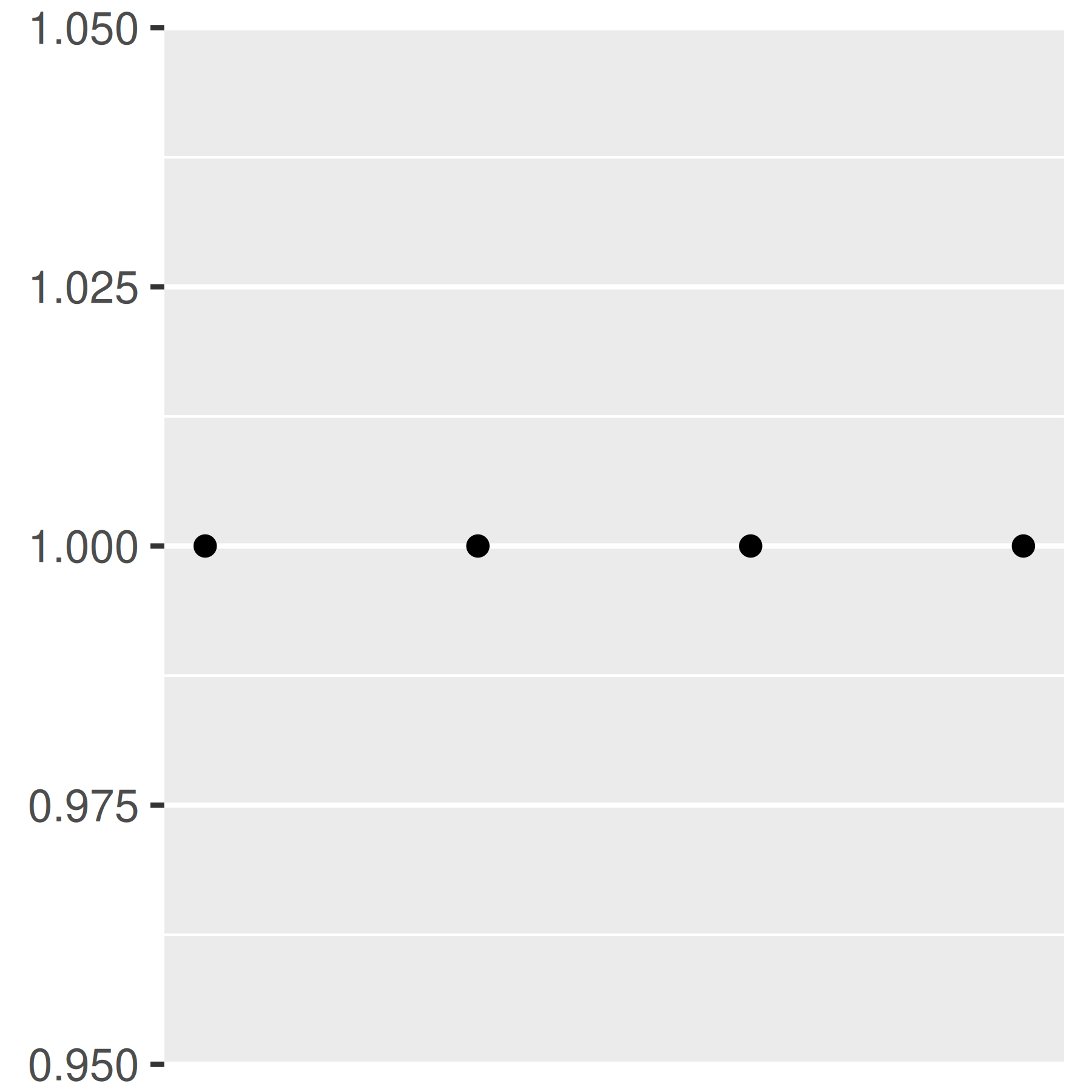
You can suppress labels with labels = NULL. This will remove the labels from the axis or legend while leaving its other properties unchanged. Notice the difference between setting breaks = NULL and labels = NULL:
base + scale_y_continuous(breaks = NULL)
base + scale_y_continuous(labels = NULL)

10.1.7 Transformations
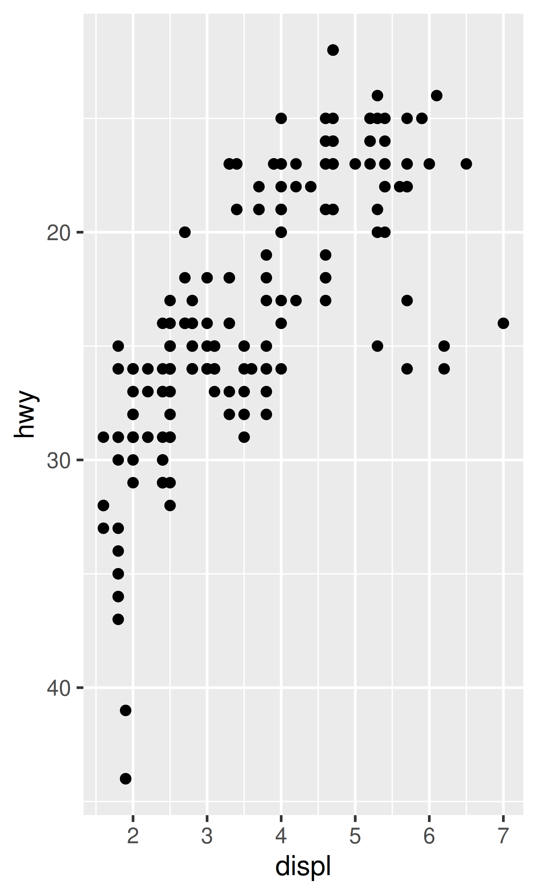
When working with continuous data, the default is to map linearly from the data space onto the aesthetic space. It is possible to override this default using scale transformations, which alter the way in which this mapping takes place. In some cases you don’t need to dive into the details, because there are convenience functions like scale_x_log10(), scale_x_reverse() that can do the work for you:
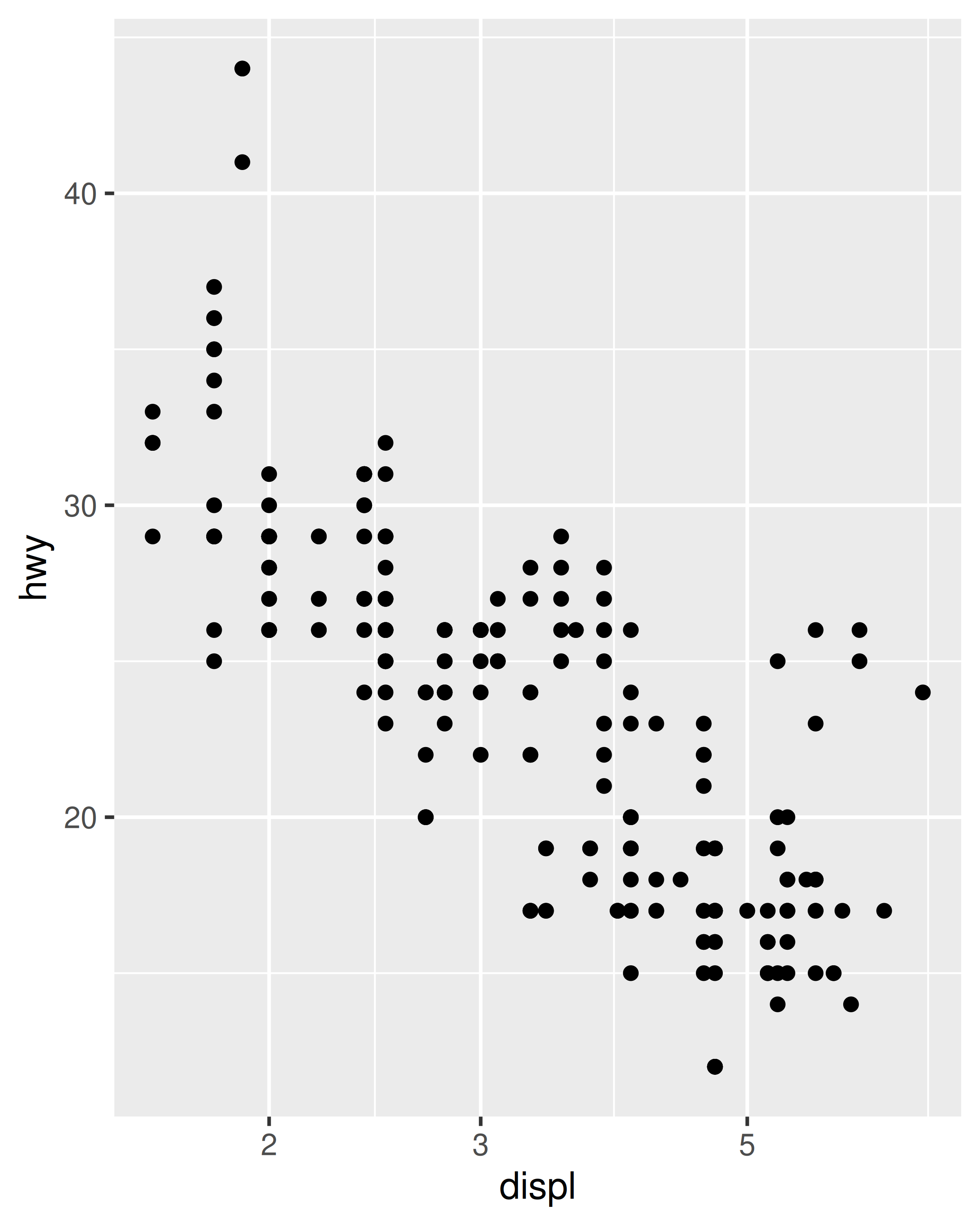
base <- ggplot(mpg, aes(displ, hwy)) + geom_point()
base
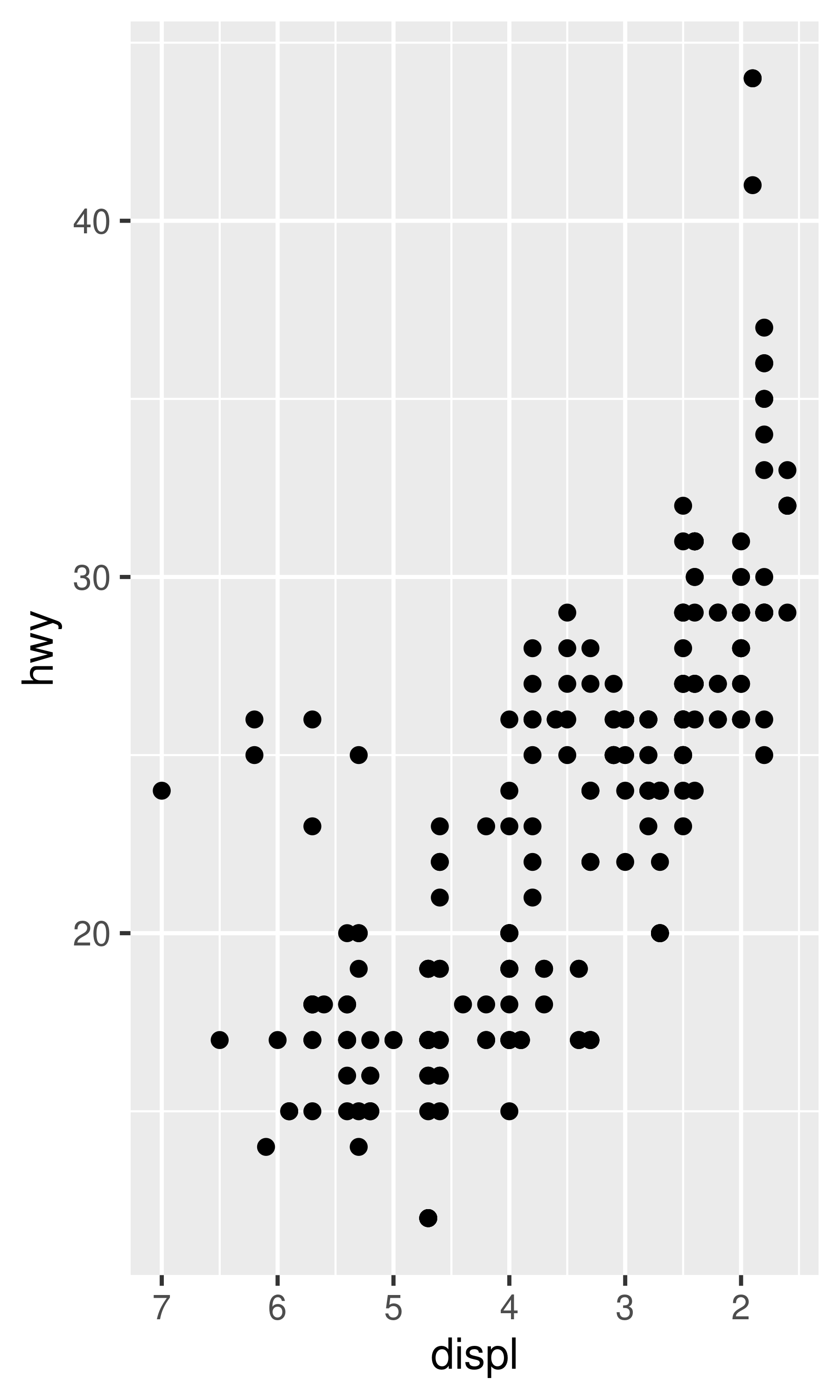
base + scale_x_reverse()
base + scale_y_reverse()
However, even in these cases a deeper understanding can be valuable. Every continuous scale takes a trans argument, allowing the use of a variety of transformations:
# convert from fuel economy to fuel consumption
ggplot(mpg, aes(displ, hwy)) +
  geom_point() +
  scale_y_continuous(trans = "reciprocal")

# log transform x and y axes
ggplot(diamonds, aes(price, carat)) +
  geom_bin2d() +
  scale_x_continuous(trans = "log10") +
  scale_y_continuous(trans = "log10")
#> `stat_bin2d()` using `bins = 30`. Pick better value `binwidth`.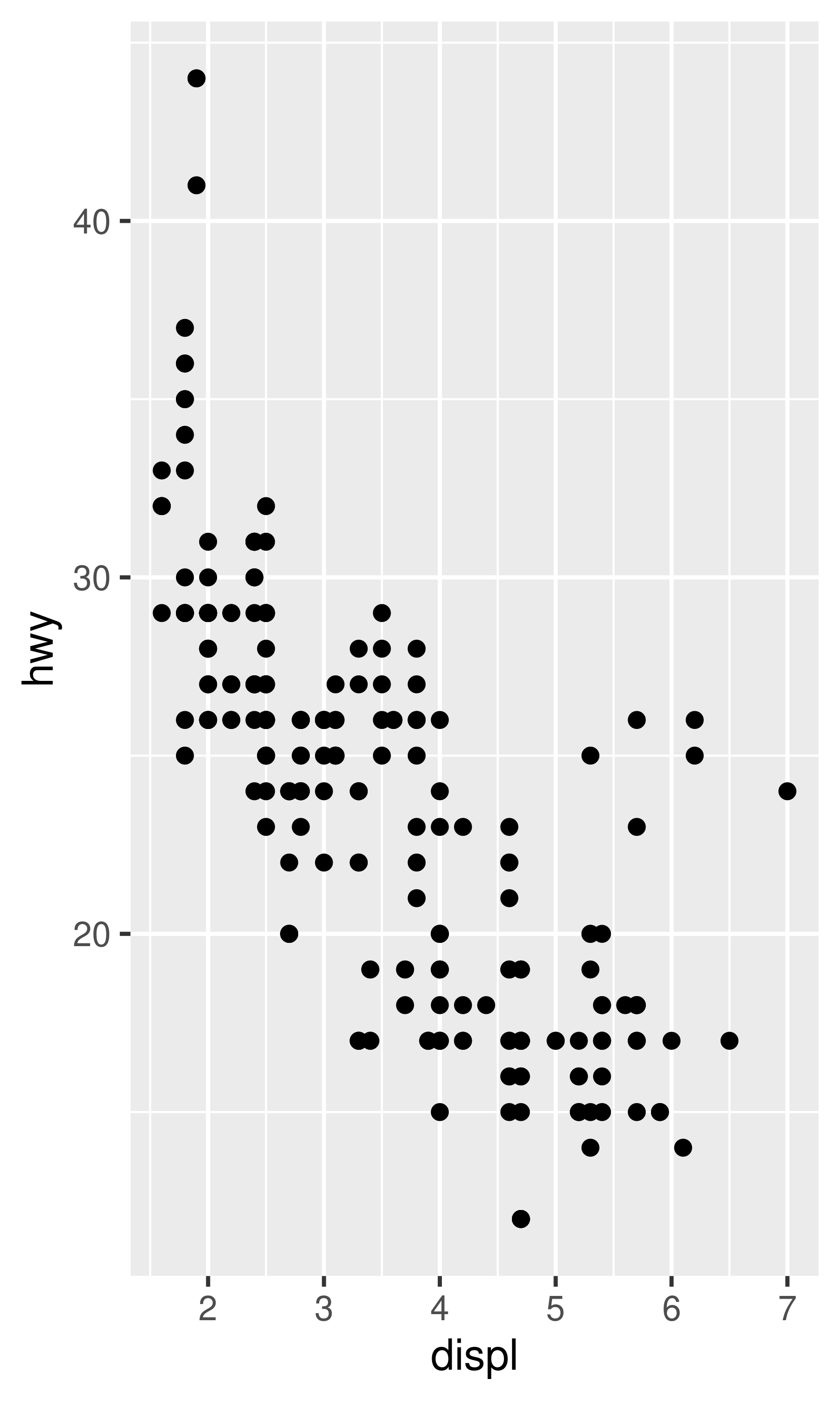
The transformation is carried out by a “transformer”, which describes the transformation, its inverse, and how to draw the labels. You can construct your own transformer using scales::trans_new(), but as the plots above illustrate, ggplot2 understands many common transformations supplied by the scales package. The following table lists some of the more common variants:
| Name | Transformer | Function \(f(x)\) | Inverse \(f^{-1}(x)\) |
|---|---|---|---|
"asn" |
scales::asn_trans() |
\(\tanh^{-1}(x)\) | \(\tanh(y)\) |
"exp" |
scales::exp_trans() |
\(e ^ x\) | \(\log(y)\) |
"identity" |
scales::identity_trans() |
\(x\) | \(y\) |
"log" |
scales::log_trans() |
\(\log(x)\) | \(e ^ y\) |
"log10" |
scales::log10_trans() |
\(\log_{10}(x)\) | \(10 ^ y\) |
"log2" |
scales::log2_trans() |
\(\log_2(x)\) | \(2 ^ y\) |
"logit" |
scales::logit_trans() |
\(\log(\frac{x}{1 - x})\) | \(\frac{1}{1 + e(y)}\) |
"probit" |
scales::probit_trans() |
\(\Phi(x)\) | \(\Phi^{-1}(y)\) |
"reciprocal" |
scales::reciprocal_trans() |
\(x^{-1}\) | \(y^{-1}\) |
"reverse" |
scales::reverse_trans() |
\(-x\) | \(-y\) |
"sqrt" |
scales::scale_x_sqrt() |
\(x^{1/2}\) | \(y ^ 2\) |
You can specify the trans argument as a string containing the name of the transformation, or by calling the transformer directly. The following are equivalent:
ggplot(mpg, aes(displ, hwy)) +
  geom_point() +
  scale_y_continuous(trans = "reciprocal")

ggplot(mpg, aes(displ, hwy)) +
  geom_point() +
  scale_y_continuous(trans = scales::reciprocal_trans())
In a few cases ggplot2 simplifies this even further, and provides convenience functions for the most common transformations: scale_x_log10(), scale_x_sqrt() and scale_x_reverse() provide the relevant transformation on the x axis, with similar functions provided for the y axis. Thus, these two plot specifications are also equivalent:
ggplot(diamonds, aes(price, carat)) +
  geom_bin2d() +
  scale_x_continuous(trans = "log10") +
  scale_y_continuous(trans = "log10")
#> `stat_bin2d()` using `bins = 30`. Pick better value `binwidth`.

ggplot(diamonds, aes(price, carat)) +
  geom_bin2d() +
  scale_x_log10() +
  scale_y_log10()
#> `stat_bin2d()` using `bins = 30`. Pick better value `binwidth`.
Note that there is nothing preventing you from performing these transformations manually. For example, instead of using scale_x_log10() to transform the scale, you could transform the data instead and plot log10(x). The appearance of the geom will be the same, but the tick labels will be different. Specifically, if you use a transformed scale, the axes will be labelled in the original data space; if you transform the data, the axes will be labelled in the transformed space. As a consequence, these plot specifications are slightly different:
# manual transformation
ggplot(mpg, aes(log10(displ), hwy)) +
  geom_point()

# transform using scales
ggplot(mpg, aes(displ, hwy)) +
  geom_point() +
  scale_x_log10()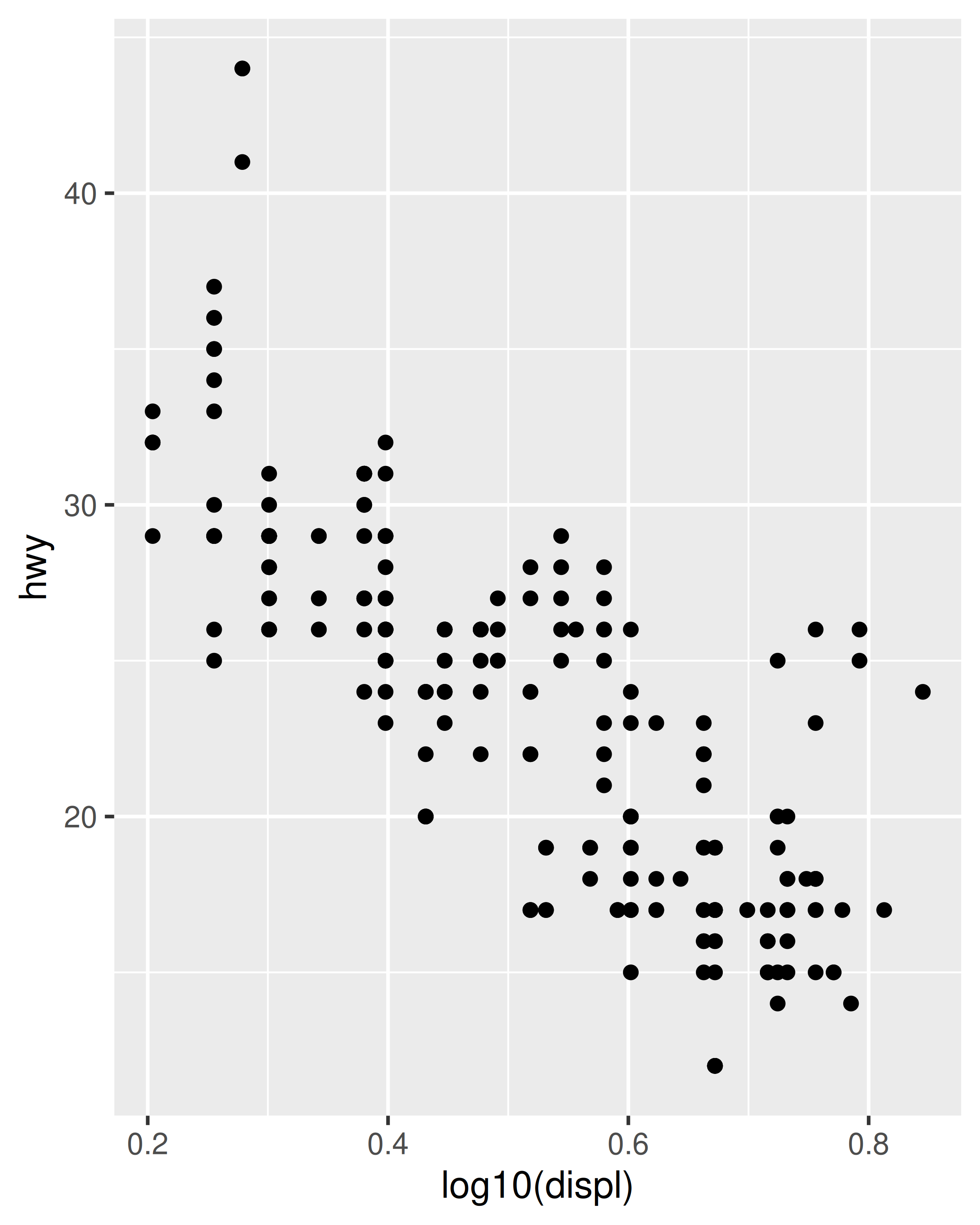
Regardless of which method you use, the transformation occurs before any statistical summaries. To transform after statistical computation use coord_trans(). See Section 15.1 for more details on coordinate systems, and Section 14.6 if you need to transform something other than a numeric position scale.
10.2 Date-time position scales
A special case of numeric position arises when an aesthetic is mapped to a date/time type. Examples of date/time types include the base Date (for dates) and POSIXct (for date-times) classes, as well as the hms class for “time of day” values provided by the hms package (Müller 2020). If your dates are in a different format you will need to convert them using as.Date(), as.POSIXct() or hms::as_hms(). You may also find the lubridate package helpful to manipulate date/time data (Grolemund and Wickham 2011).
Assuming you have appropriately formatted data mapped to the x aesthetic, ggplot2 will use scale_x_date() as the default scale for dates and scale_x_datetime() as the default scale for date-time data. The corresponding scales for other aesthetics follow the usual naming rules. Date scales behave similarly to other continuous scales, but contain additional arguments that allow you to work in date-friendly units. This section discusses date/time scales for position aesthetics: see Section 11.5 for colour and fill aesthetics.
10.2.1 Breaks
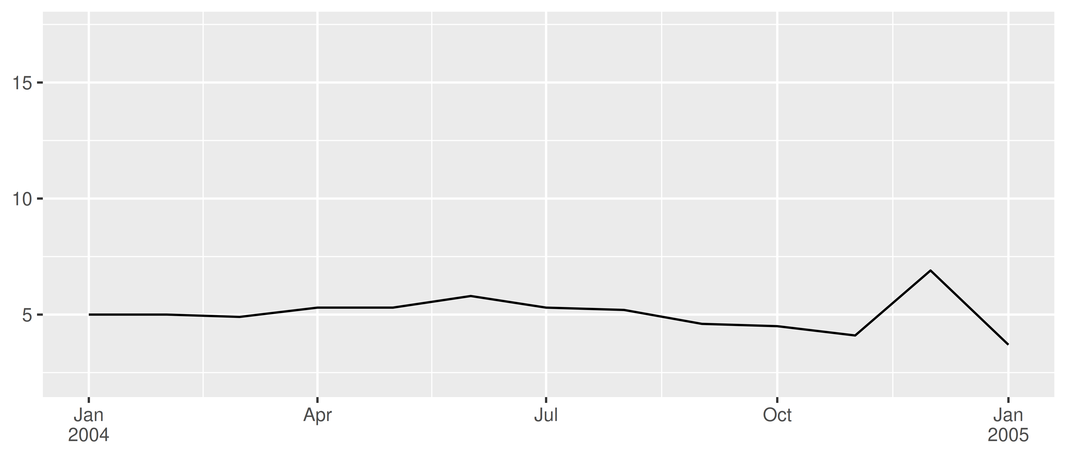
The date_breaks argument allows you to position breaks by date units (years, months, weeks, days, hours, minutes, and seconds). For example, date_breaks = "2 weeks" will place a major tick mark every two weeks and date_breaks = "15 years" will place them every 15 years:
date_base <- ggplot(economics, aes(date, psavert)) +
  geom_line(na.rm = TRUE) +
  labs(x = NULL, y = NULL)

date_base
date_base + scale_x_date(date_breaks = "15 years")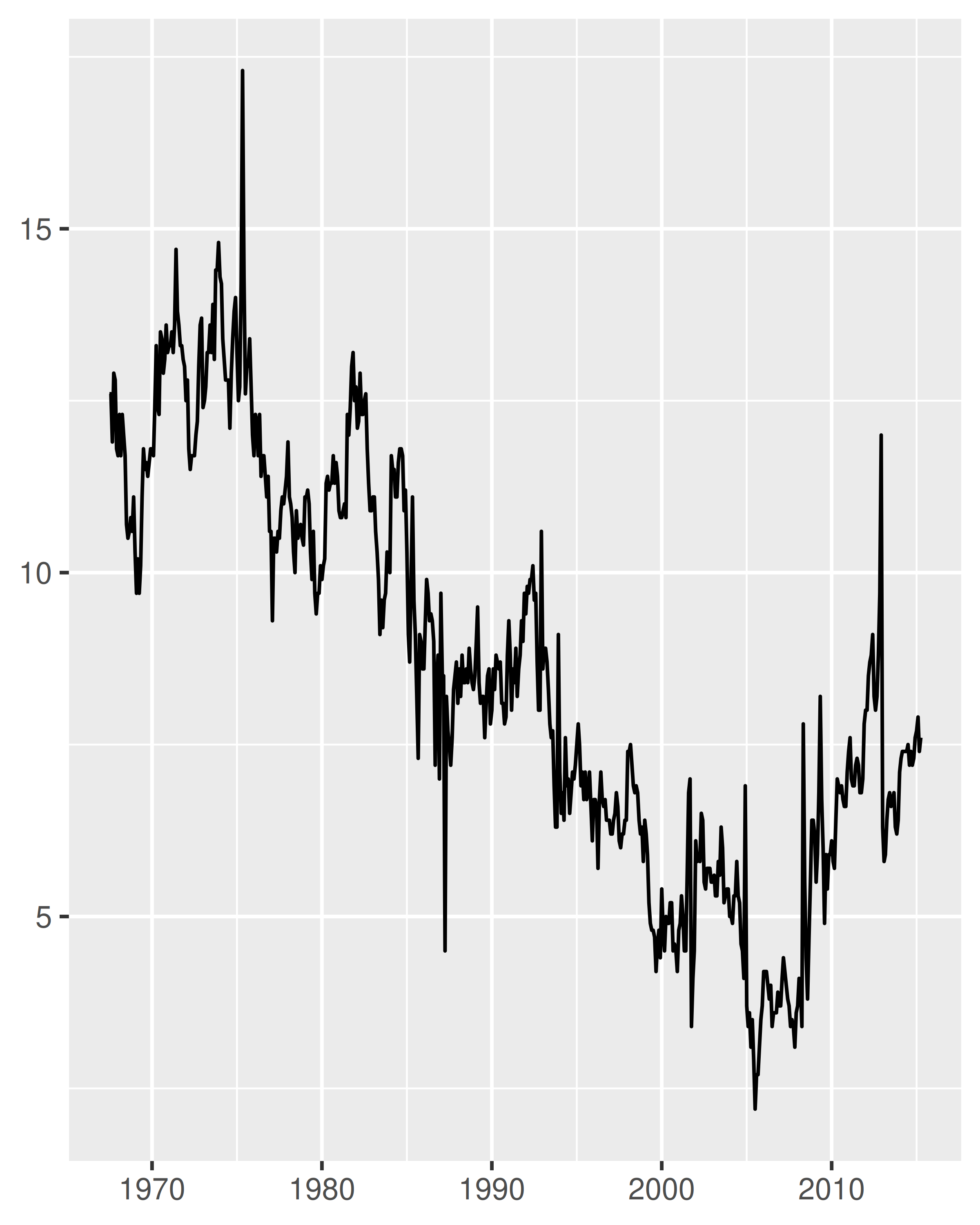
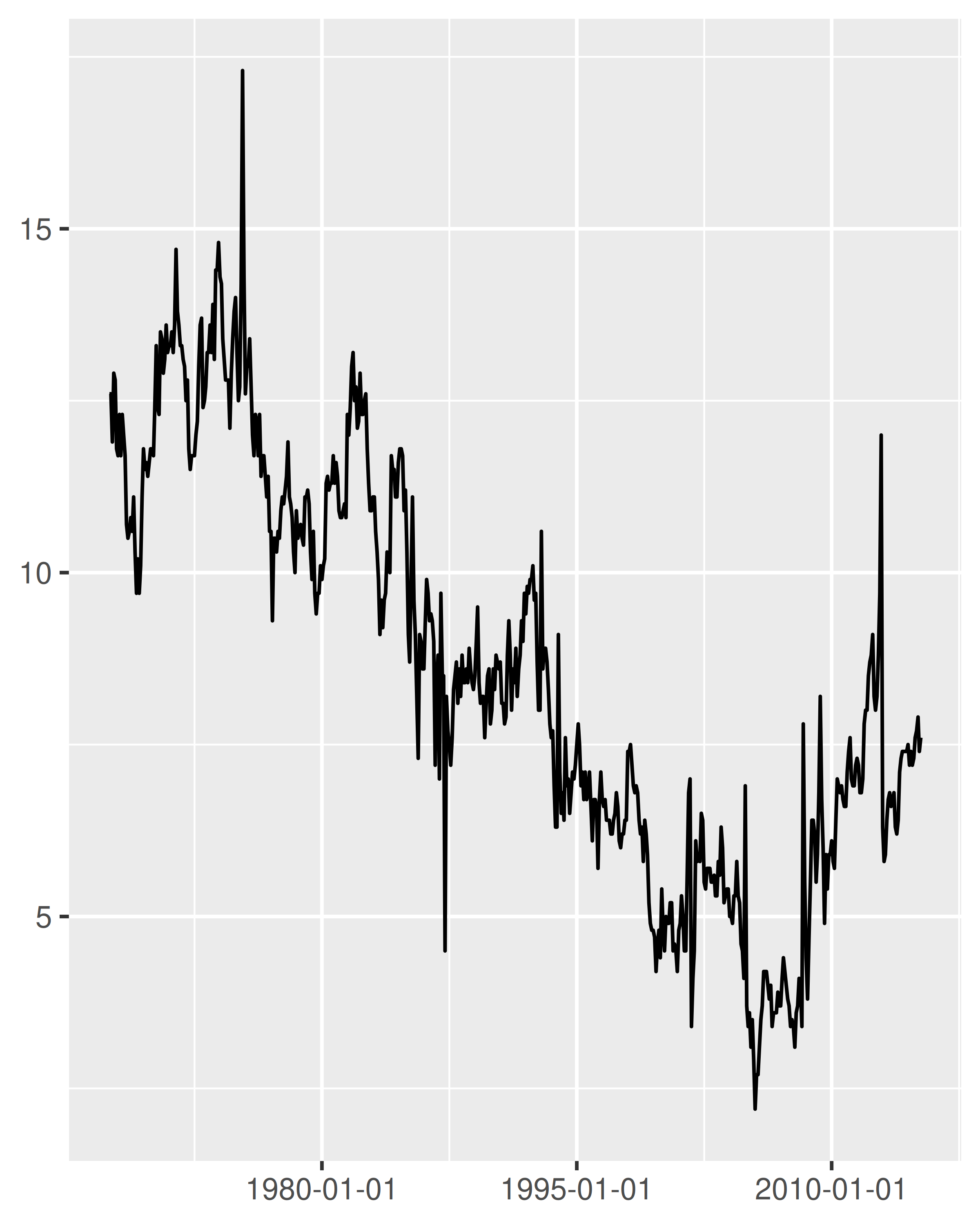
Compared to the plot on the left, two things have changed in the plot on the right: the tick marks are placed at 15 year intervals, and the label format has changed. We’ll discuss date labelling in Section 10.2.3, but for now our focus is on the breaks.
To understand how ggplot2 interprets date_breaks = "15 years", it is helpful to note that it is merely a convenient shorthand for setting breaks = scales::breaks_width("15 years"). The longer form is typically unnecessary, but it can be useful if—as discussed in Section 10.1.4—you wish to specify an offset. For example, suppose the goal is to plot data spanning a calendar year, with monthly breaks. Specifying date_breaks = "1 month" is equivalent to setting scales::breaks_width("1 month"), which produces these breaks:
the_year <- as.Date(c("2021-01-01", "2021-12-31"))
set_breaks <- scales::breaks_width("1 month")
set_breaks(the_year)
#>  [1] "2021-01-01" "2021-02-01" "2021-03-01" "2021-04-01" "2021-05-01"
#>  [6] "2021-06-01" "2021-07-01" "2021-08-01" "2021-09-01" "2021-10-01"
#> [11] "2021-11-01" "2021-12-01" "2022-01-01"
In this example, the set_breaks() function returned by scales::break_width() produces breaks spaced one month apart, where the date for each break falls on the first day of the month. Placing each break at the start of the calendar year is usually sensible, but there are exceptions. Perhaps the data track income and expenses for a household in which a monthly salary is paid on the ninth day of each month. In this situation it may be sensible to have the breaks aligned with the salary deposits. To do this, we can set offset = 8 when we define the set_breaks() function:
set_breaks <- scales::breaks_width("1 month", offset = 8)
set_breaks(the_year)
#>  [1] "2021-01-09" "2021-02-09" "2021-03-09" "2021-04-09" "2021-05-09"
#>  [6] "2021-06-09" "2021-07-09" "2021-08-09" "2021-09-09" "2021-10-09"
#> [11] "2021-11-09" "2021-12-09" "2022-01-09"
10.2.2 Minor breaks
Date/times scales also have a date_minor_breaks argument that allows you to specify the minor breaks in using date units, in exactly the same fashion that date_breaks does for major breaks. To illustrate this, we’ll define an empty plot with a date scale on the y-axis, and tweak the theme (Chapter 17) to make the grid lines more visually prominent:
df <- data.frame(y = as.Date(c("2022-01-01", "2022-04-01")))
base <- ggplot(df, aes(y = y)) +
  labs(y = NULL) +
  theme_minimal() +
  theme(
    panel.grid.major = element_line(colour = "black"),
    panel.grid.minor = element_line(colour = "grey50")
  )

base + scale_y_date(date_breaks = "1 month")
base +
  scale_y_date(date_breaks = "1 month", date_minor_breaks = "1 week")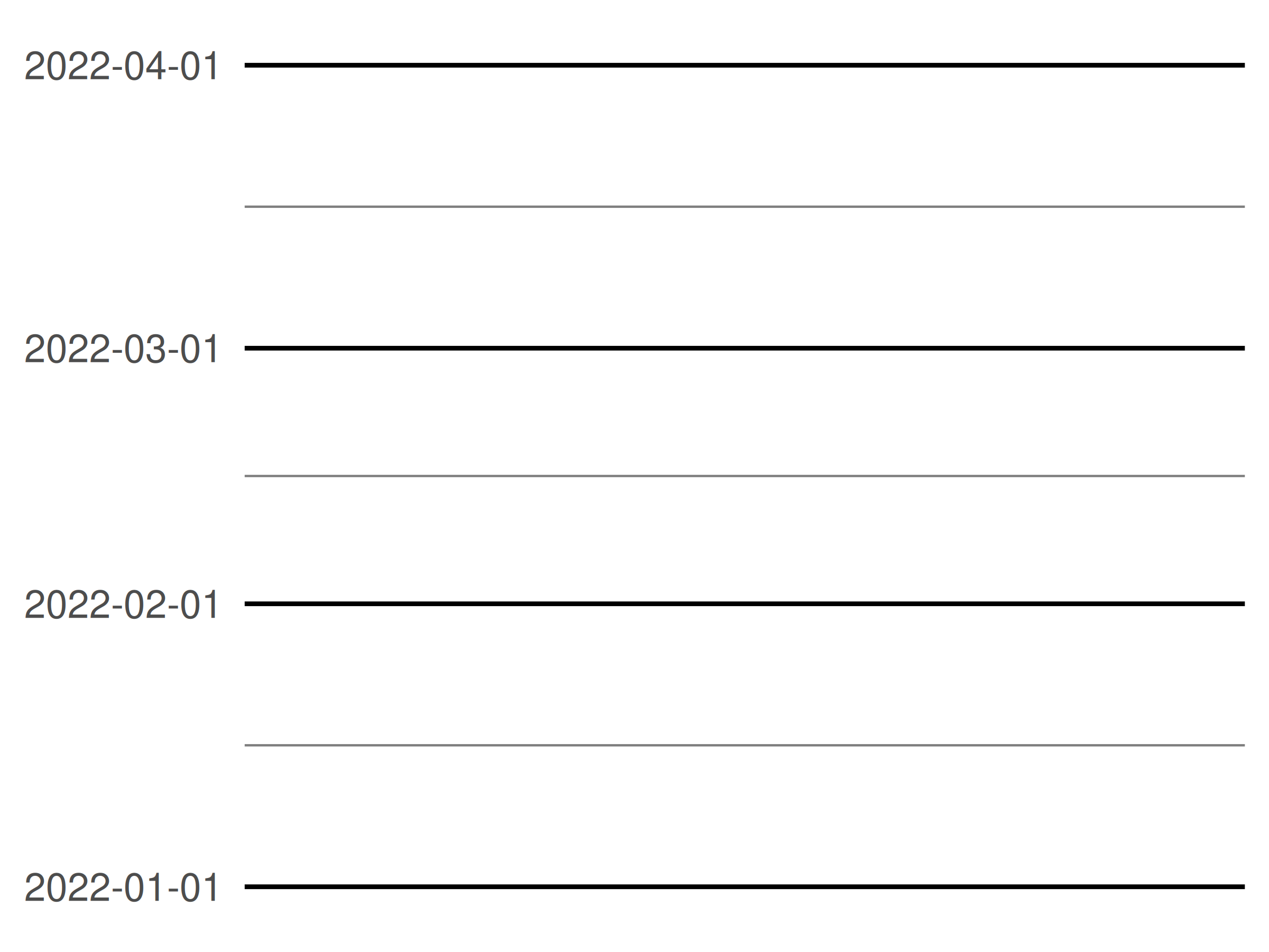
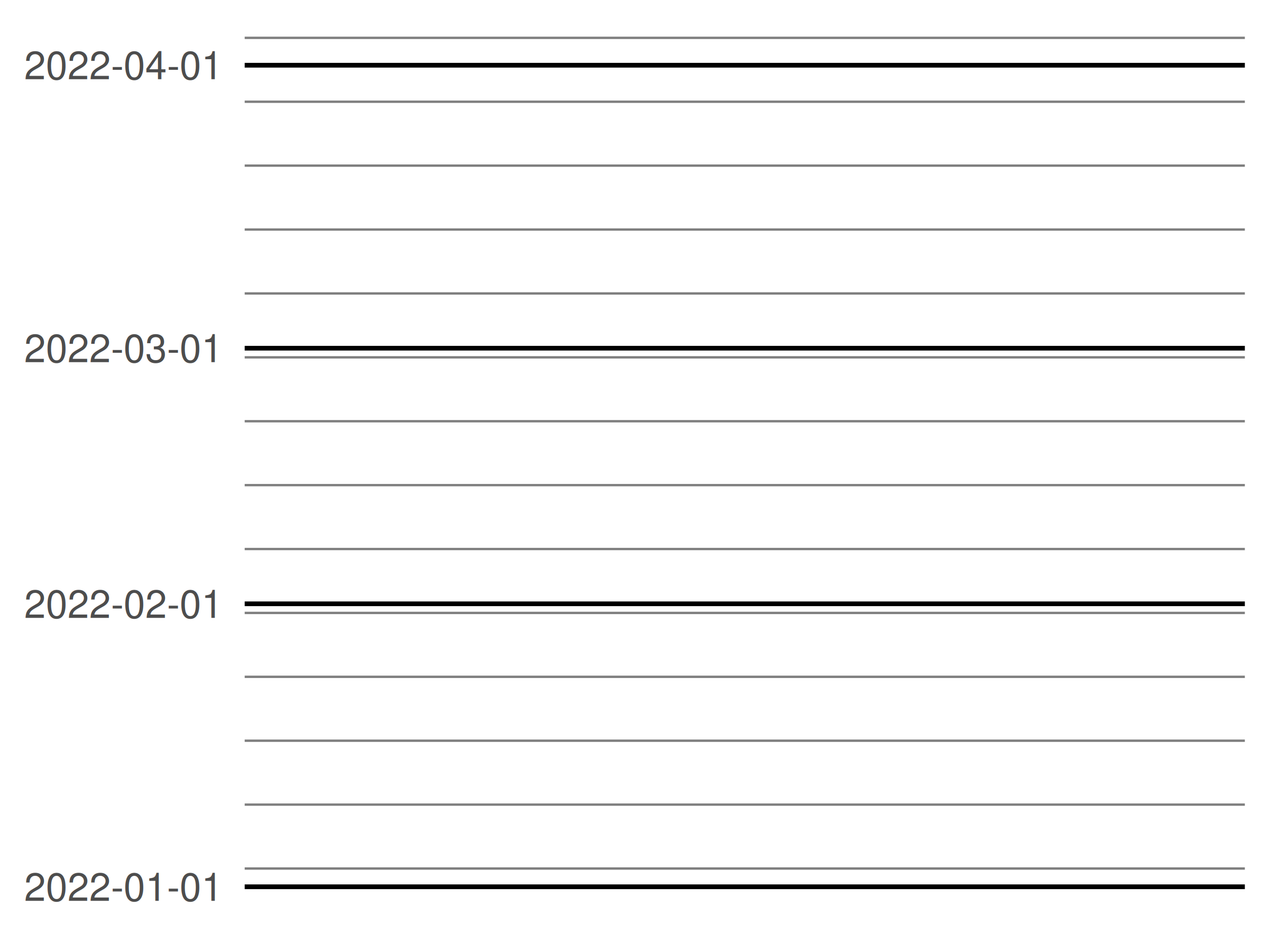
Note that in the first plot, the minor breaks are spaced evenly between the monthly major breaks. In the second plot, the major and minor breaks follow slightly different patterns: the minor breaks are always spaced 7 days apart but the major breaks are 1 month apart. Because the months vary in length, this leads to slightly uneven spacing.
10.2.3 Labels
Date scales contain a labels argument that behaves similarly to the corresponding argument for numeric scales, but is often more convenient to use the date_labels argument. It controls the display of the labels using the same formatting strings as in strptime() and format(). To display dates like 14/10/1979, for example, you would use the string "%d/%m/%Y": in this expression %d produces a numeric day of month, %m produces a numeric month, and %Y produces a four-digit year. The table below provides a list of formatting strings:
| String | Meaning |
|---|---|
%S |
second (00-59) |
%M |
minute (00-59) |
%l |
hour, in 12-hour clock (1-12) |
%I |
hour, in 12-hour clock (01-12) |
%p |
am/pm |
%H |
hour, in 24-hour clock (00-23) |
%a |
day of week, abbreviated (Mon-Sun) |
%A |
day of week, full (Monday-Sunday) |
%e |
day of month (1-31) |
%d |
day of month (01-31) |
%m |
month, numeric (01-12) |
%b |
month, abbreviated (Jan-Dec) |
%B |
month, full (January-December) |
%y |
year, without century (00-99) |
%Y |
year, with century (0000-9999) |
One useful scenario for date label formatting is when there’s insufficient room to specify a four-digit year. Using %y ensures that only the last two digits are displayed:
base <- ggplot(economics, aes(date, psavert)) +
  geom_line(na.rm = TRUE) +
  labs(x = NULL, y = NULL)

base + scale_x_date(date_breaks = "5 years")
base + scale_x_date(date_breaks = "5 years", date_labels = "%y")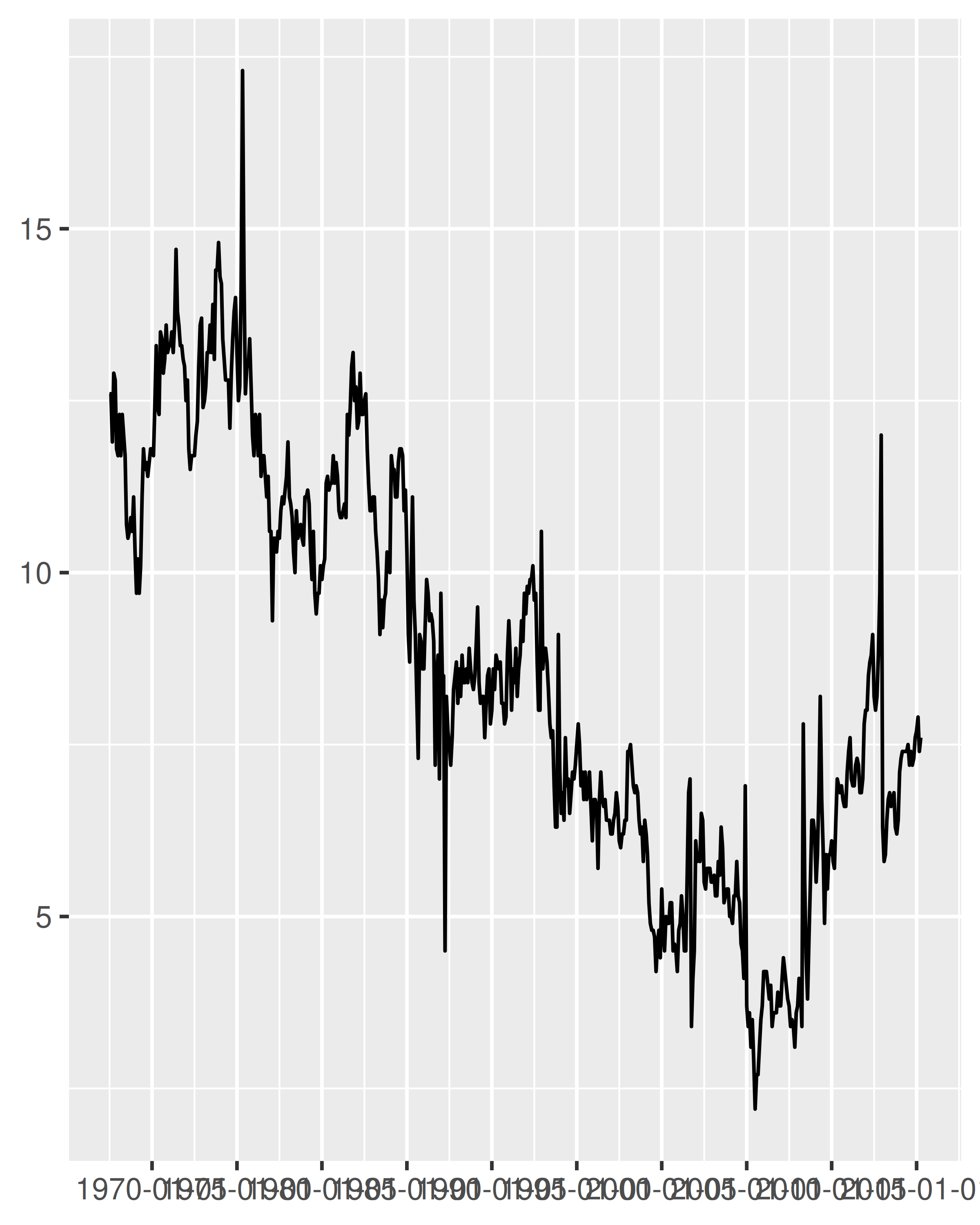

It can be useful to include the line break character \n in a formatting string, particularly when full-length month names are included:
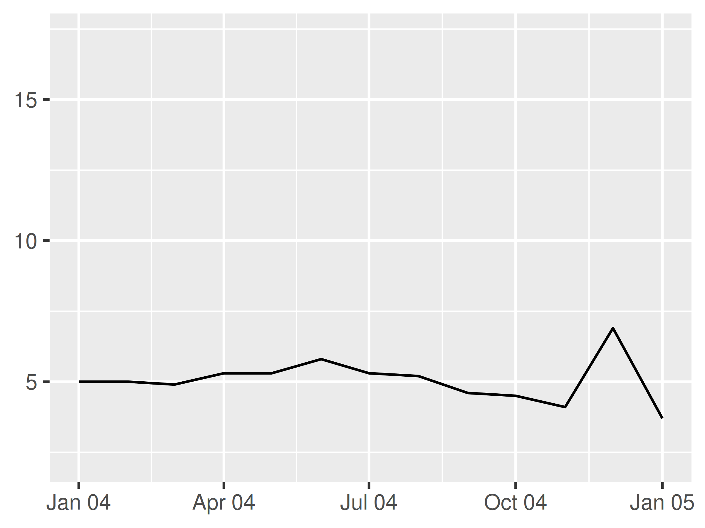
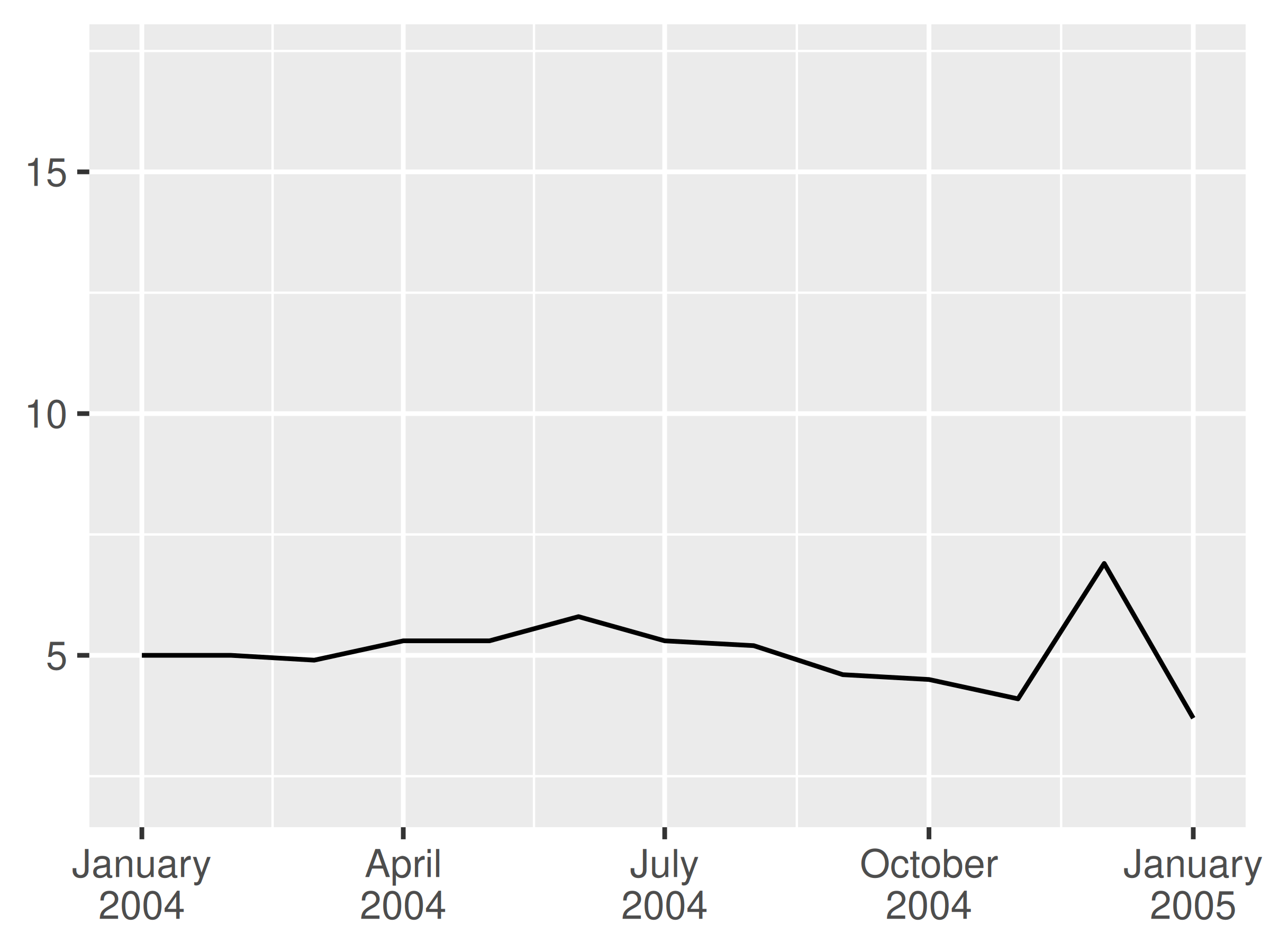
In these examples we have specified the labels manually via the date_labels argument. An alternative approach is to pass a labelling function to the labels argument, in the same way we described in Section 10.1.6. You can write your own custom labelling function, but this is often unnecessary. The scales package provides convenient functions that can generate labellers for you, notably scales::label_date() and scales::label_date_short(). You rarely need to call scales::label_date() directly, because that’s the function that date_labels uses. However, if you want to use scales::label_date_short() you’ll need to do so explicitly. The goal of label_date_short() is to automatically construct short labels that are sufficient to uniquely identify the dates:
base +
  scale_x_date(
    limits = lim,
    labels = scales::label_date_short()
  )
This can often produce clearer plots: in the example above each year is labelled only once rather than appearing in every label, reducing the amount of visual clutter and making it easier for the viewer to see where each year begins and ends.
10.3 Discrete position scales
It is also possible to map discrete variables to position scales, with the default scales being scale_x_discrete() and scale_y_discrete(). For example, the following two plot specifications are equivalent
ggplot(mpg, aes(x = hwy, y = class)) +
geom_point()
ggplot(mpg, aes(x = hwy, y = class)) +
geom_point() +
scale_x_continuous() +
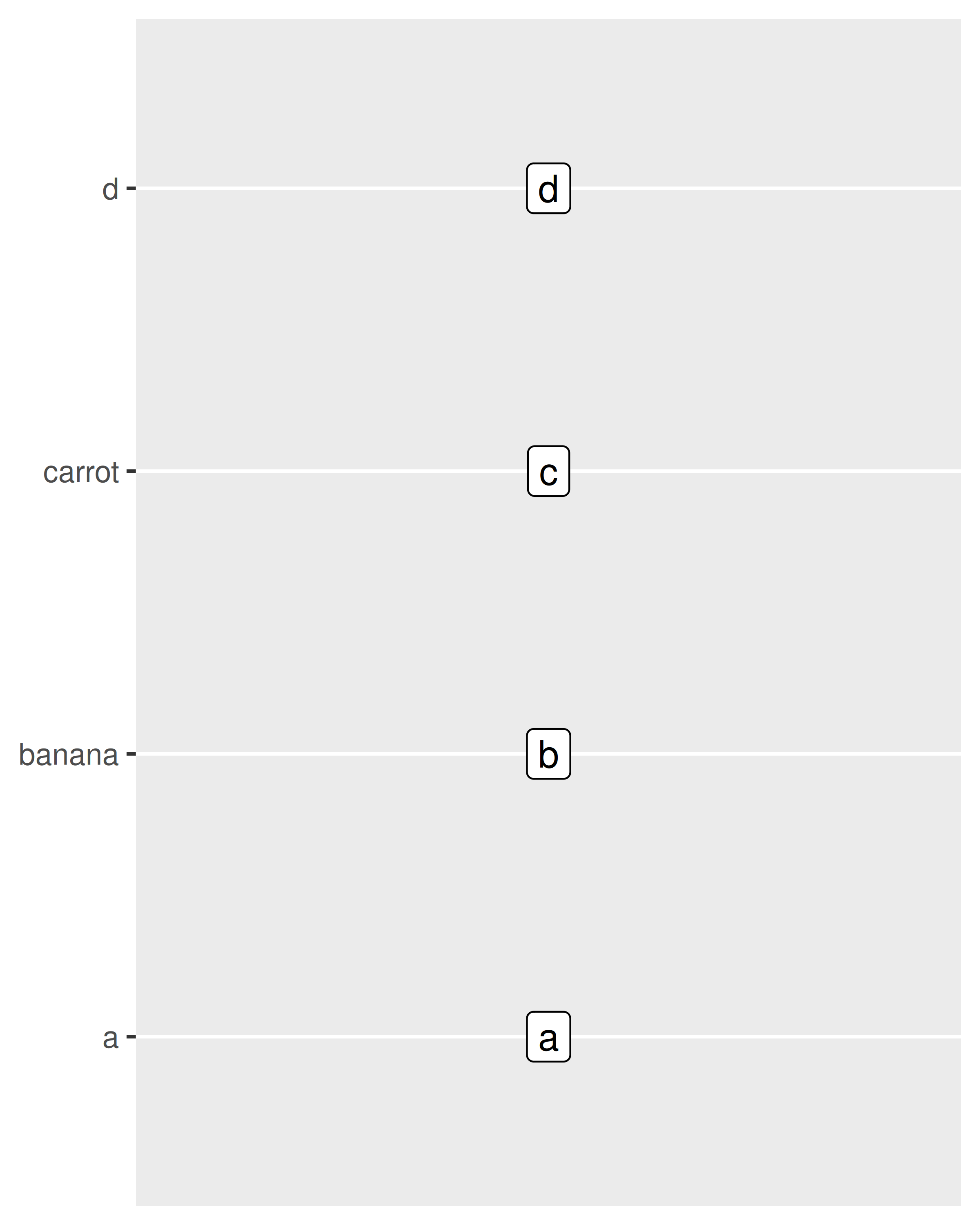
scale_y_discrete()Internally, ggplot2 handles discrete scales by mapping each category to an integer value and then drawing the geom at the corresponding coordinate location. To illustrate this, we can add a custom annotation (see Section 8.3) to the plot:
ggplot(mpg, aes(x = hwy, y = class)) +
  geom_point() +
  annotate("text", x = 5, y = 1:7, label = 1:7)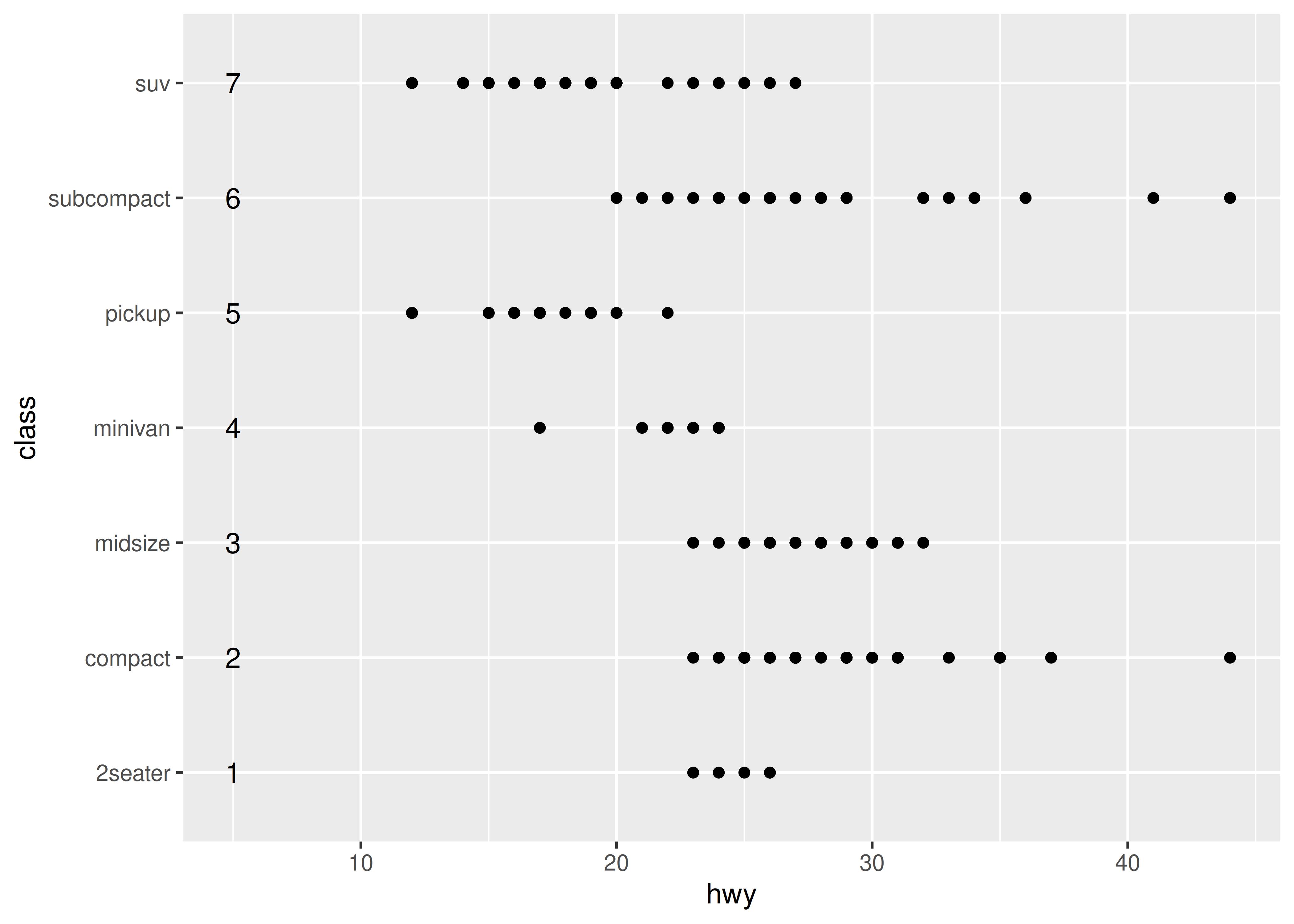
Mapping each category to an integer value is useful because it means that other width quantities can be specified as a proportion of the category range. For instance, in the preceding plot, we could specify a vertical jitter for each point spanning half the width of the implied category bin:
ggplot(mpg, aes(x = hwy, y = class)) +
  geom_jitter(width = 0, height = .25) +
  annotate("text", x = 5, y = 1:7, label = 1:7)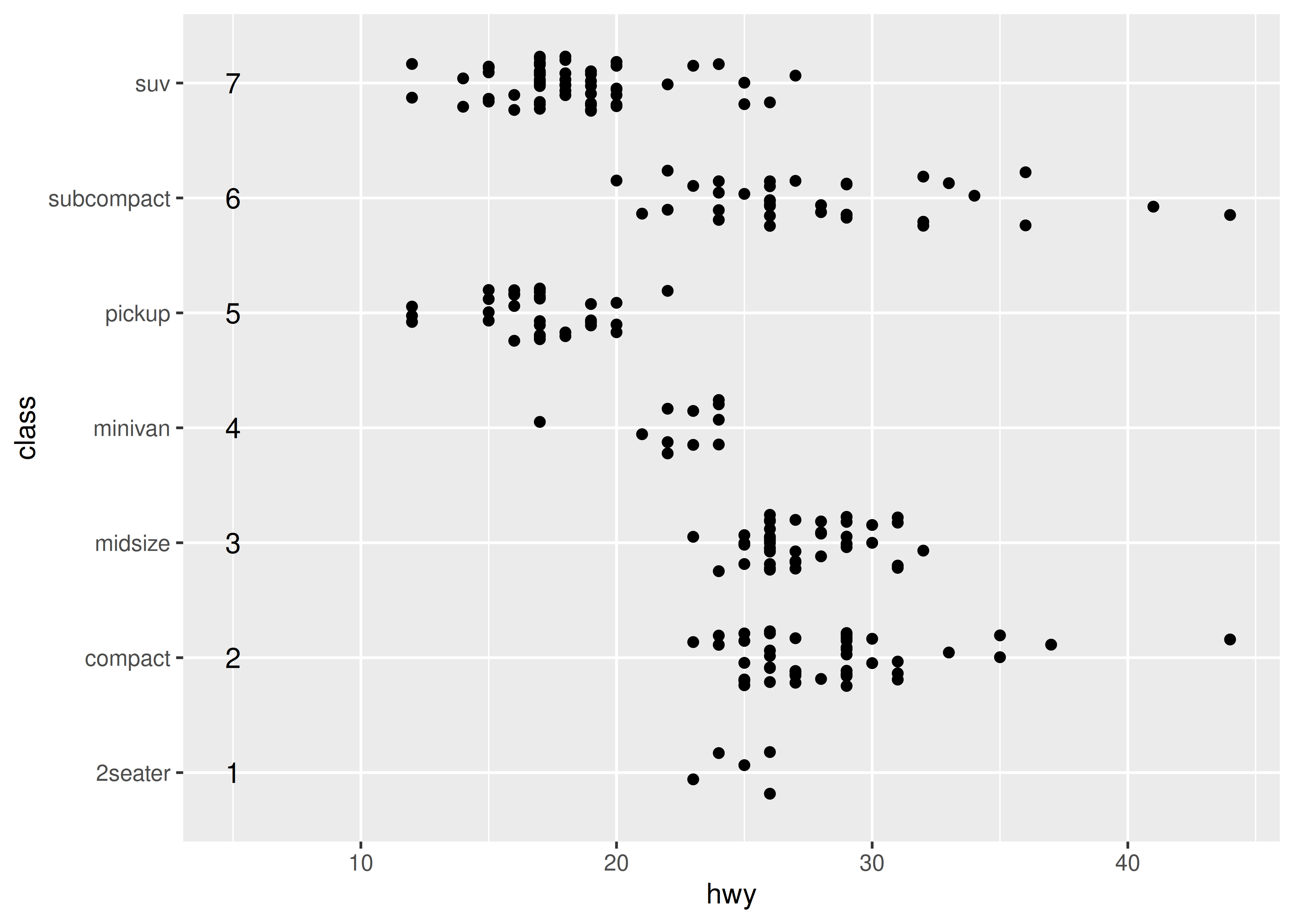
The same mechanism underpins the widths of bars and boxplots. Because each category has width 1 in a discrete scale, setting width = .4 when using geom_boxplot() ensures that the box occupies 40% of the width allocated to the category:
ggplot(mpg, aes(x = drv, y = hwy)) + geom_boxplot()
ggplot(mpg, aes(x = drv, y = hwy)) + geom_boxplot(width = .4)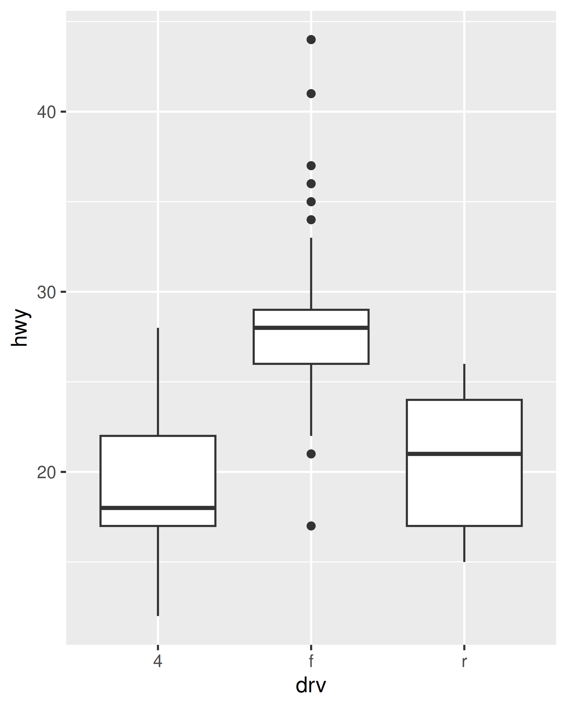
10.3.1 Limits, breaks, and labels
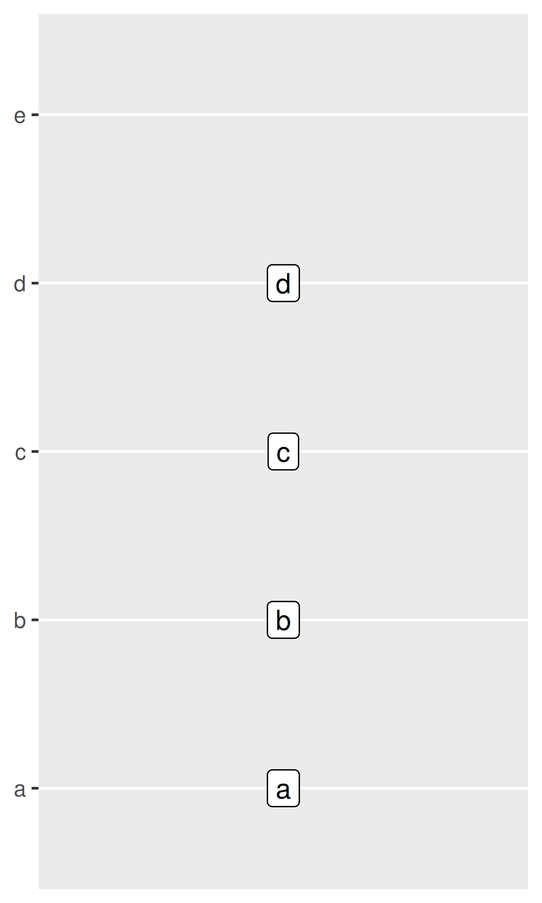
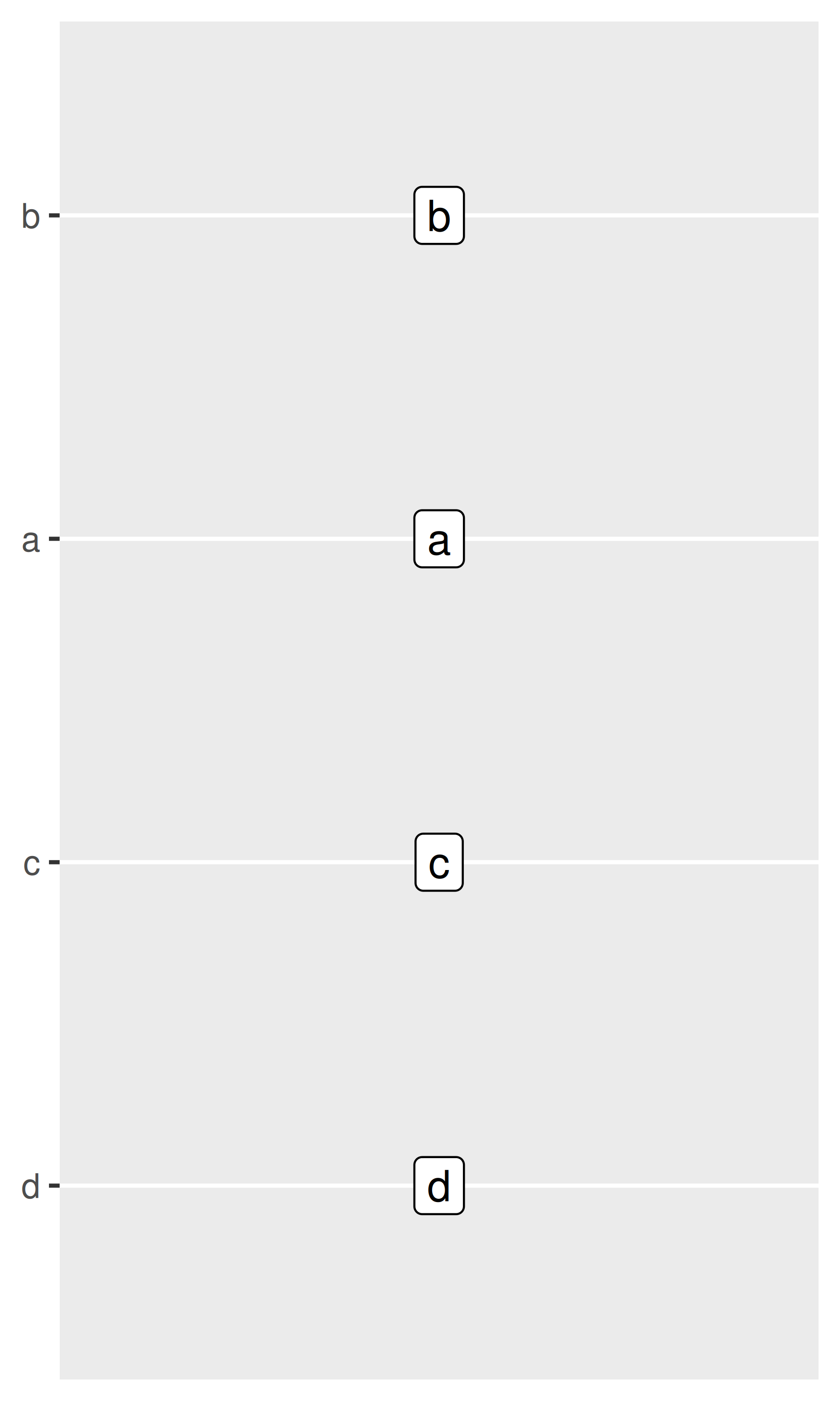
The limits, breaks. and labels for a discrete position scale can be set using the limits, breaks, and labels arguments. For the most part these behave identically to the corresponding arguments for numeric scales (Section 10.1), though there are some differences. For example, the limits of a discrete scale are not defined in terms of endpoints, but instead correspond to the set of allowable values for that variable. Accordingly, ggplot2 expects that the limits of a discrete scale should be a character vector that enumerates all possible values in the order they should appear:

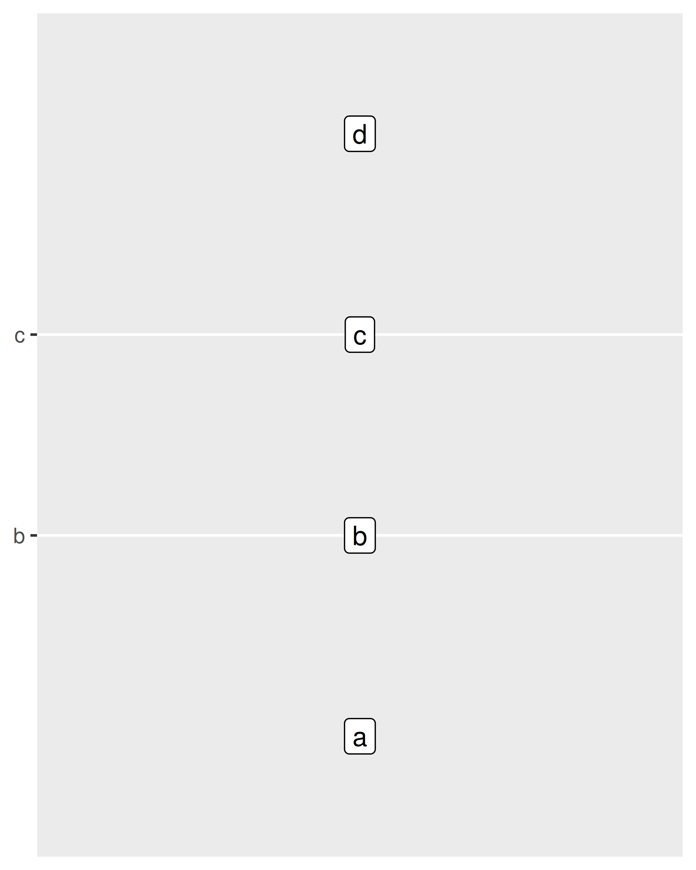
The breaks argument is largely unchanged, enumerating a set of values to be displayed on the axis labels. The labels argument for discrete scales has some additional functionality: you also have the option of using a named vector to set the labels associated with particular values. This allows you to change some labels and not others, without altering the ordering or the breaks:
As with other scales, discrete position scales allow you to pass a function to the labels argument. The scales::label_wrap() function can be particularly valuable for categorical data, as it allows you to wrap long strings across multiple lines.
10.3.2 Label positions
When plotting categorical data it is often necessary to move the axis labels in some way to prevent them from overlapping:
base <- ggplot(mpg, aes(manufacturer, hwy)) + geom_boxplot()
base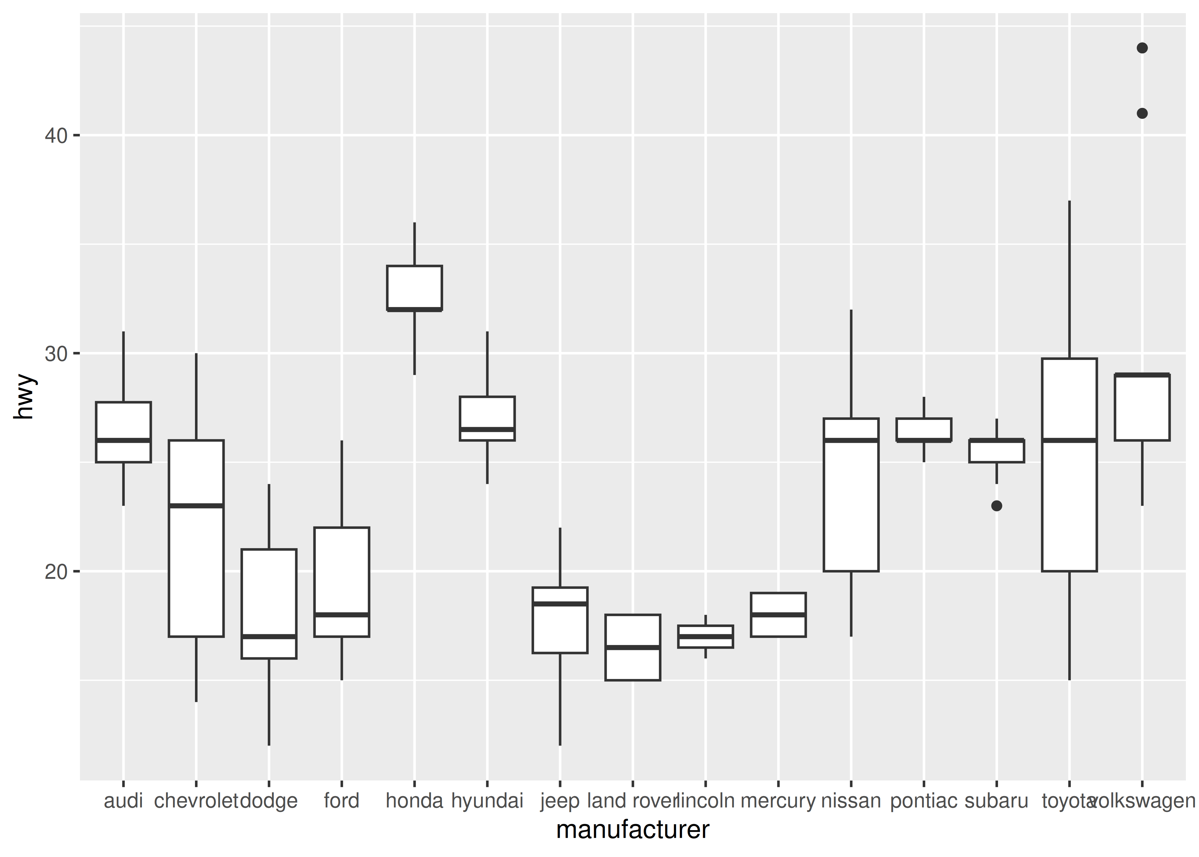
Even when allocated a lot of horizontal space, the axis labels overlap considerably on this plot. We can control this with the help of the guides() function, which works in a similar way to the labs() helper function described in Section 8.1. Both take the name of different aesthetics (e.g., color, x, fill) as arguments and allow you to specify your own value. For a position aesthetic, we use the guide_axis() to tell ggplot2 how we want to modify the axis labels. For example, we could tell ggplot2 to “dodge” the position of the labels by setting guide_axis(n.dodge = 3), or to rotate them by setting guide_axis(angle = 90):
base + guides(x = guide_axis(n.dodge = 3))
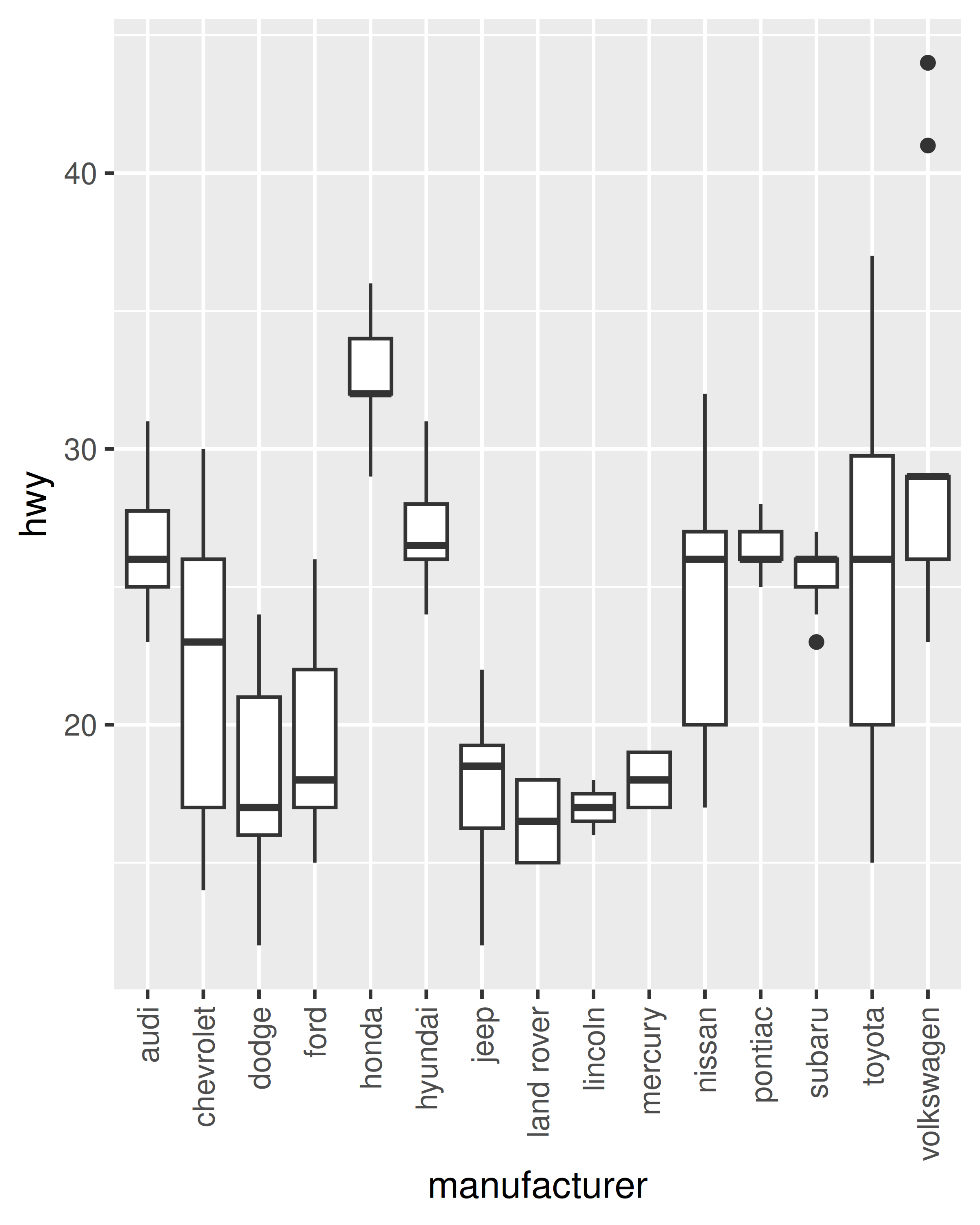
base + guides(x = guide_axis(angle = 90))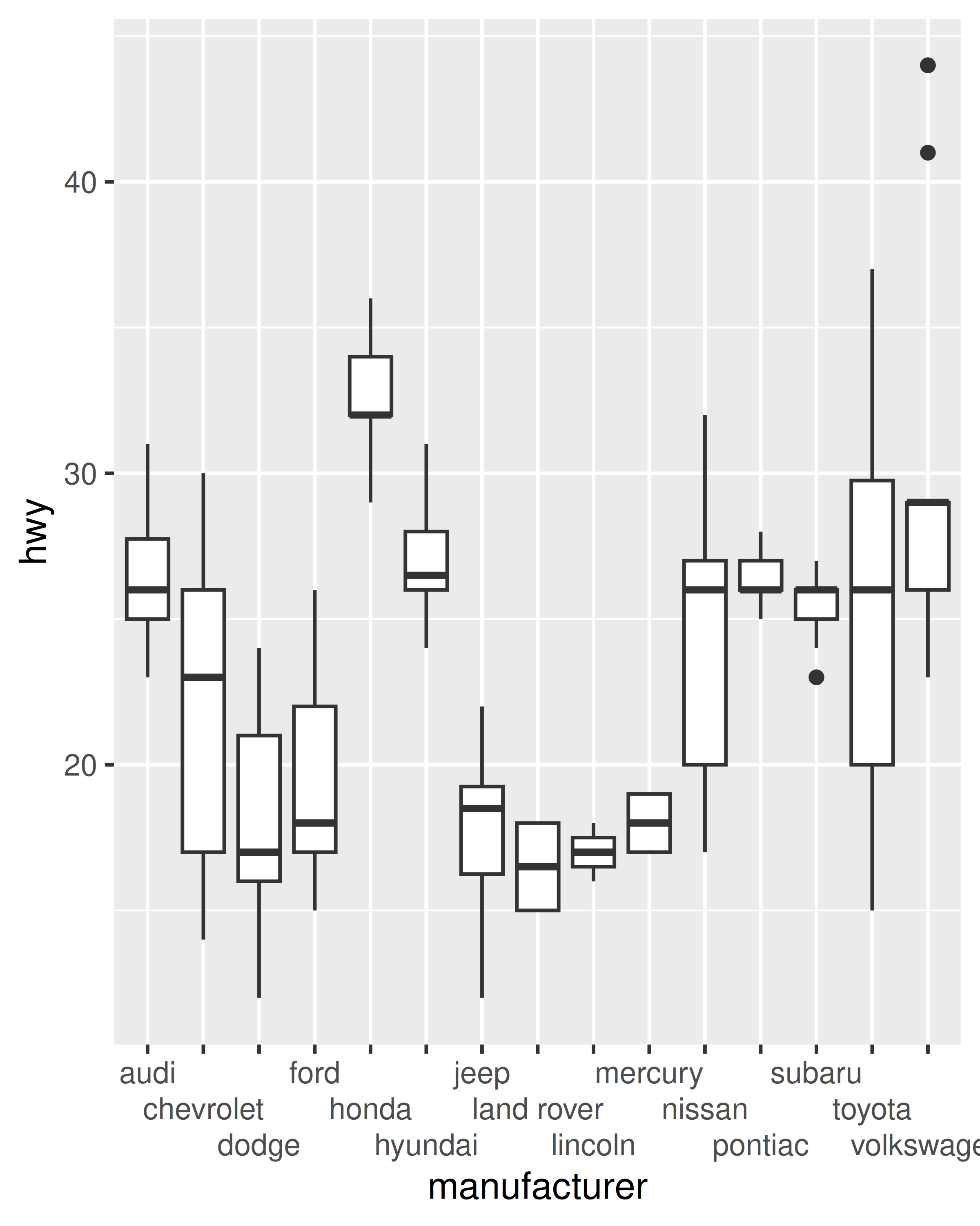
Note that, in the same way that where labs() is a shorthand way to specify the name argument to one or more scales, the guides() function is a shorthand way to set the guide arguments to one or more scales. So the code below achieves the same result:
base + scale_x_discrete(guide = guide_axis(n.dodge = 3))
base + scale_x_discrete(guide = guide_axis(angle = 90))
To learn more about guide functions see Section 14.5.
10.4 Binned position scales
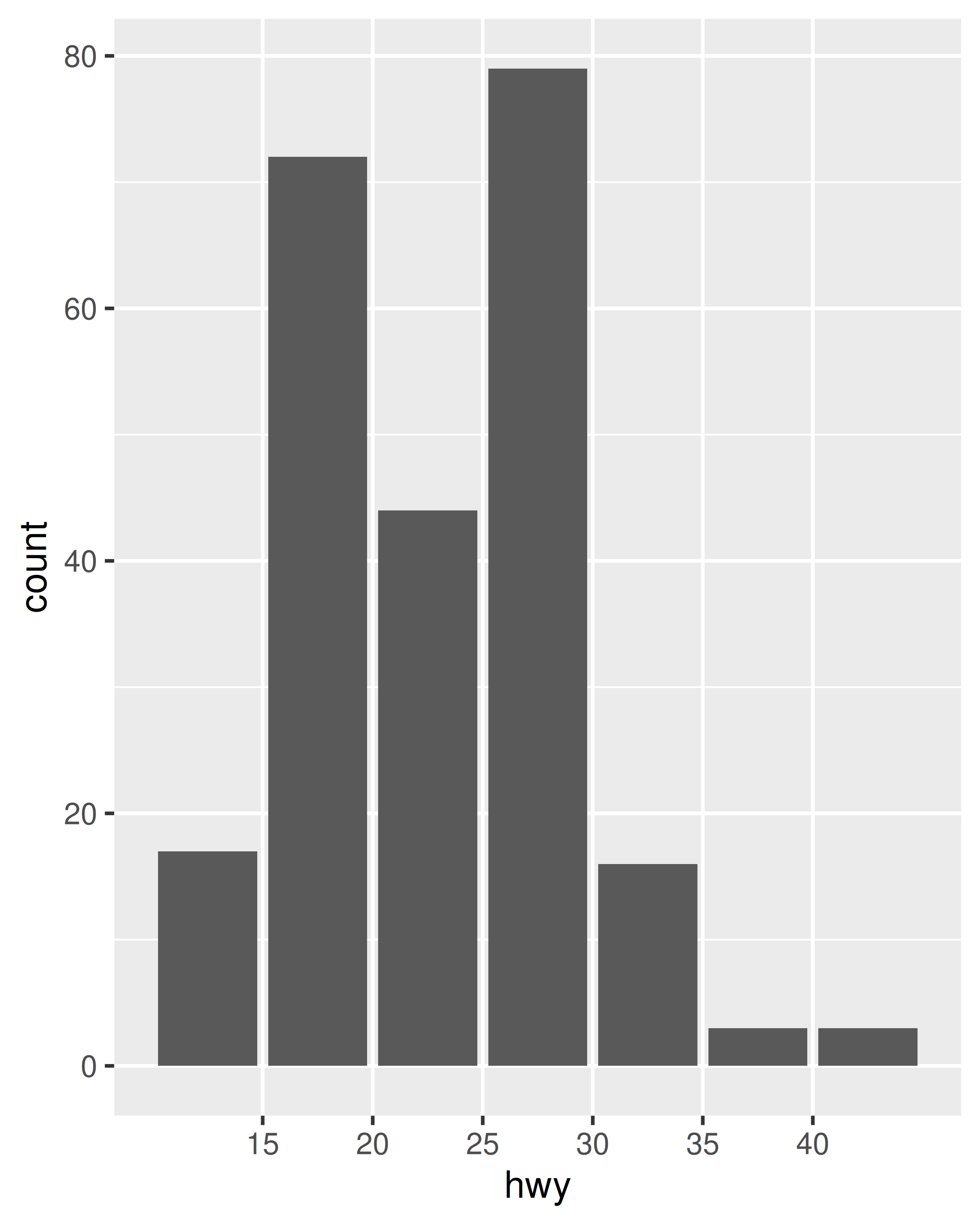
A variation on discrete position scales are binned scales, where a continuous variable is sliced into multiple bins and the discretised variable is plotted. For position aesthetics, binned scales are mostly used to create histograms and related plots. The example below shows how to approximate the behaviour of geom_histogram() using geom_bar() in combination with a binned position scale:
ggplot(mpg, aes(hwy)) + geom_histogram(bins = 8)
ggplot(mpg, aes(hwy)) +
  geom_bar() +
scale_x_binned() 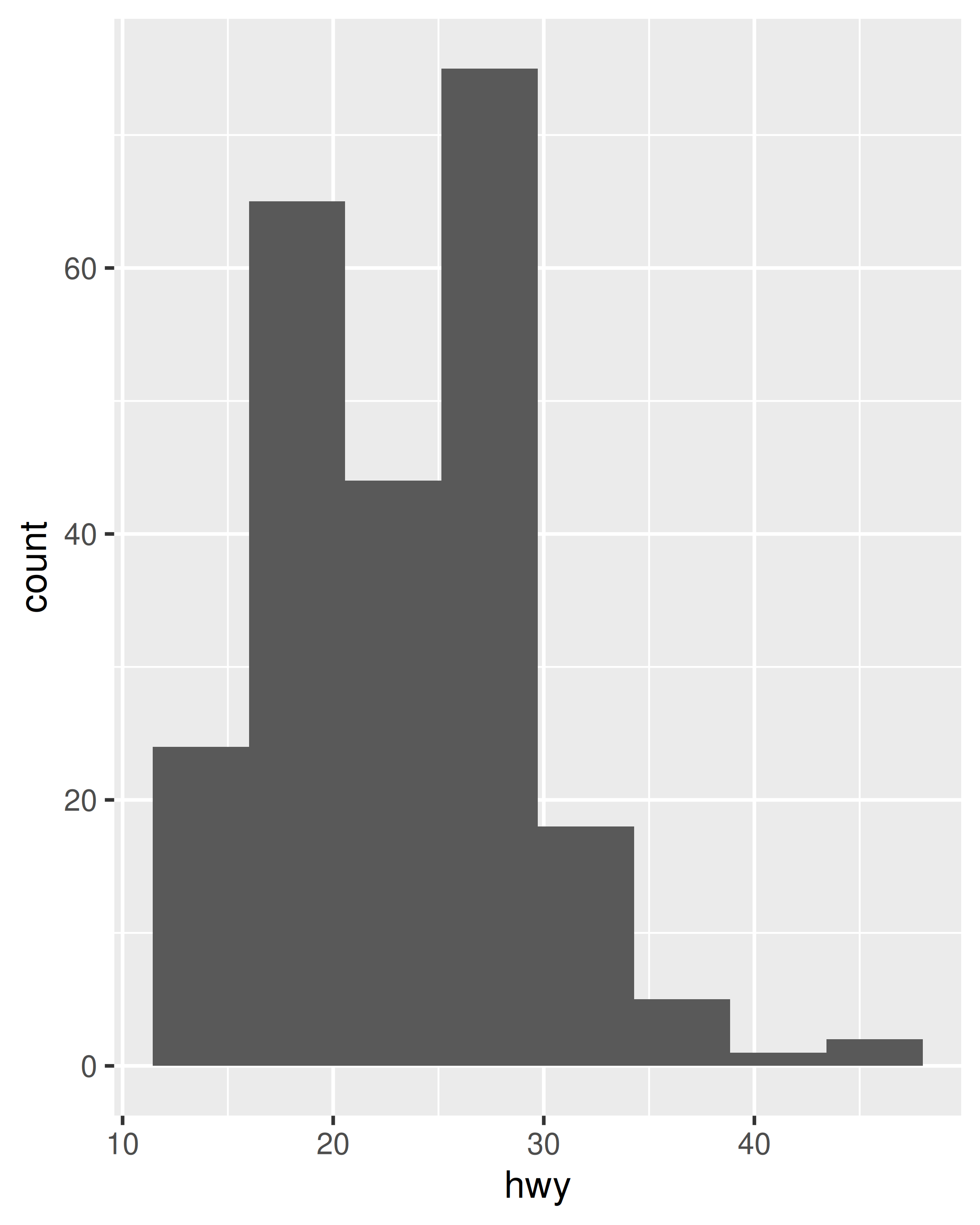
In practice this is not the most useful example, since geom_histogram() already exists and supplies defaults that are generally more appropriate for histograms, but the technique can be extended. Suppose we want to use geom_count() in place of geom_point() in order to show the number of observations at each location. The advantage of geom_count() is that the size of each dot scales with the number of observations at each location, but as the figure below illustrates, this method doesn’t work very well when data vary continuously:
base <- ggplot(mpg, aes(displ, hwy)) +
  geom_count()

base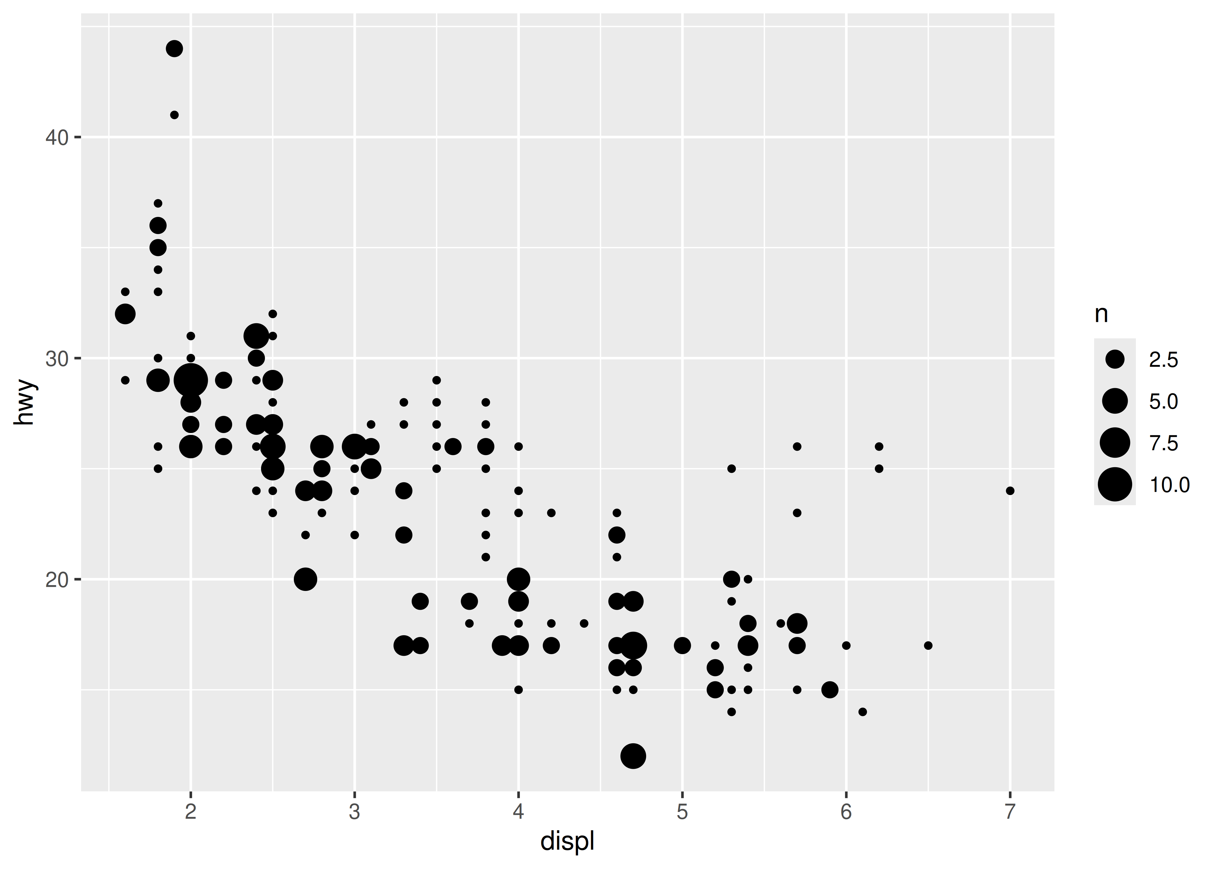
This plot is rather cluttered, and not particularly easy to read. To improve this, we can use scale_x_binned() to cut the values into bins before passing them to the geom:
base +
  scale_x_binned(n.breaks = 15) +
  scale_y_binned(n.breaks = 15)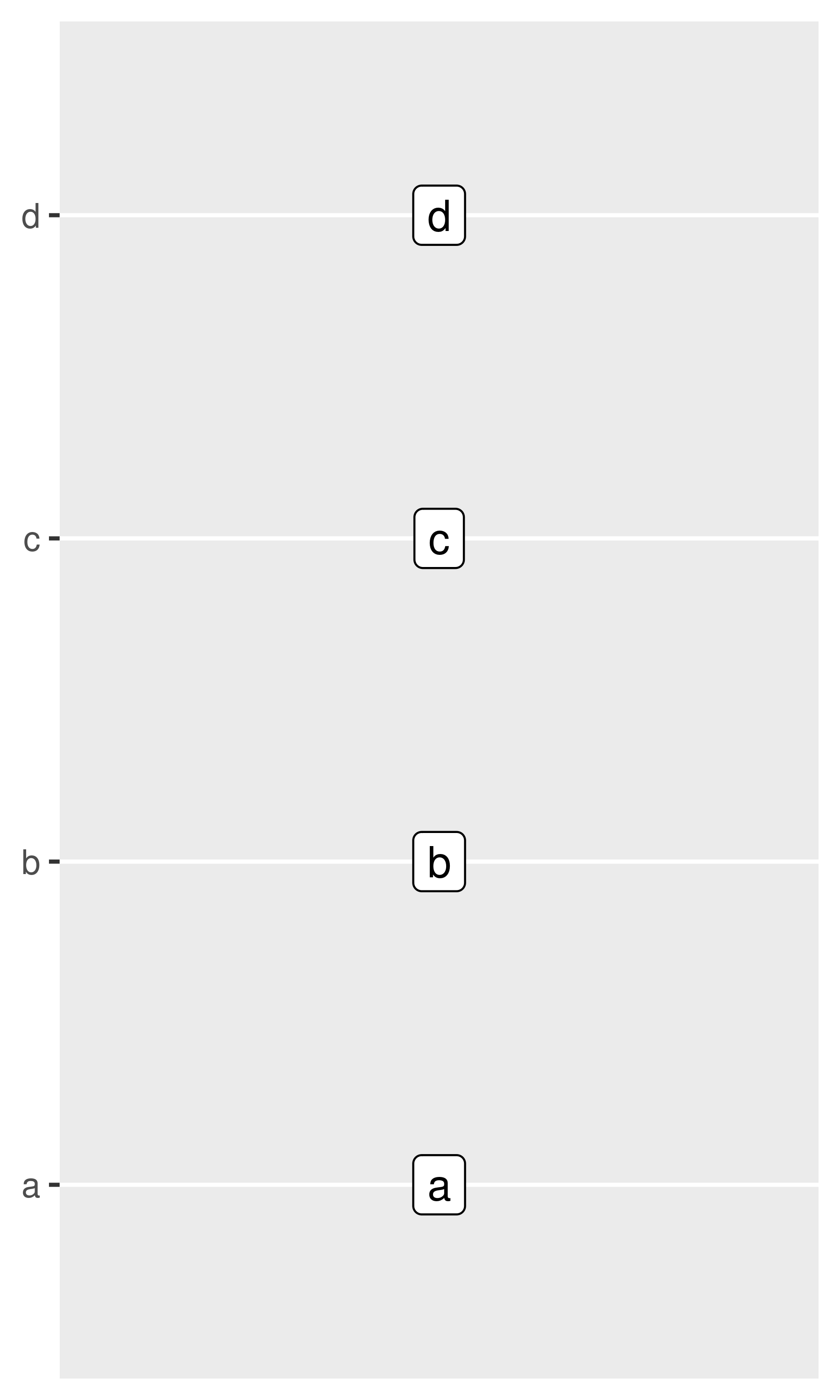
You can read more about how binned scales are used for non-position aesthetics in Section 11.4 and Section 12.1.2.
Grolemund, Garrett, and Hadley Wickham. 2011. “Dates and Times Made Easy with lubridate.” Journal of Statistical Software 40 (3): 1–25. http://www.jstatsoft.org/v40/i03/.
Müller, Kirill. 2020. Hms: Pretty Time of Day. https://CRAN.R-project.org/package=hms.
Wickham, Hadley, and Dana Seidel. 2020. Scales: Scale Functions for Visualization. https://CRAN.R-project.org/package=scales.