p <- ggplot(mpg, aes(displ, hwy, color = drv)) +
  geom_point(position = "jitter") +
  geom_smooth(method = "lm", formula = y ~ x) +
  facet_wrap(vars(year)) +
ggtitle("A plot for expository purposes")19 Internals of ggplot2
You are reading the work-in-progress third edition of the ggplot2 book. This chapter should be readable but is currently undergoing final polishing.
Throughout this book we have described ggplot2 from the perspective of a user rather than a developer. From the user point of view, the important thing is to understand how the interface to ggplot2 works. To make a data visualisation the user needs to know how functions like ggplot() and geom_point() can be used to specify a plot, but very few users need to understand how ggplot2 translates this plot specification into an image. For a ggplot2 developer who hopes to design extensions, however, this understanding is paramount.
When making the jump from user to developer, it is common to encounter frustrations because the nature of the ggplot2 interface is very different to the structure of the underlying machinery that makes it work. As extending ggplot2 becomes more common, so too does the frustration related to understanding how it all fits together. This chapter is dedicated to providing a description of how ggplot2 works “behind the curtains”. We focus on the design of the system rather than technical details of its implementation, and the goal is to provide a conceptual understanding of how the parts fit together. We begin with a general overview of the process that unfolds when a ggplot object is plotted, and then dive into details, describing how the data flows through this whole process and ends up as visual elements in your plot.
19.1 The plot() method
To understand the machinery underpinning ggplot2, it is important to recognise that almost everything related to the plot drawing happens when you print the ggplot object, not when you construct it. For instance, in the code below, the object p is an abstract specification of the plot data, the layers, etc. It does not construct the image itself:
ggplot2 is designed this way to allow the user to add new elements to a plot without needing to recalculate anything. One implication of this is that if you want to understand the mechanics of ggplot2, you have to follow your plot as it goes down the plot()1 rabbit hole. You can inspect the print method for ggplot objects by typing ggplot2:::plot.ggplot at the console, but for this chapter we will work with a simplified version. Stripped to its bare essentials, the ggplot2 plot method has the same structure as the following ggprint() function:
ggprint <- function(x) {
  data <- ggplot_build(x)
  gtable <- ggplot_gtable(data)
  grid::grid.newpage()
  grid::grid.draw(gtable)
  return(invisible(x))
}
This function does not handle every possible use case, but it is sufficient to draw the plot specified above:
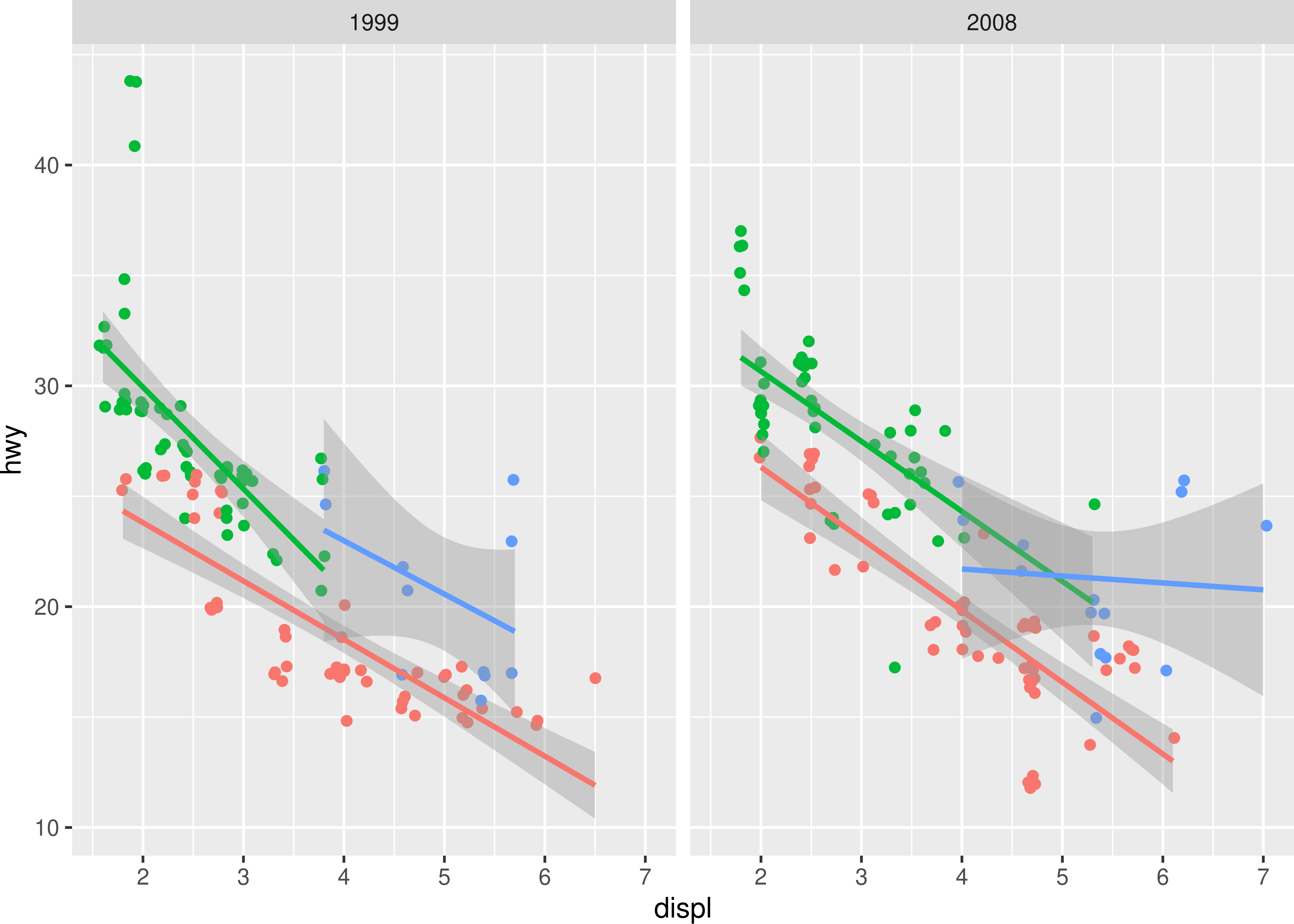
ggprint(p) 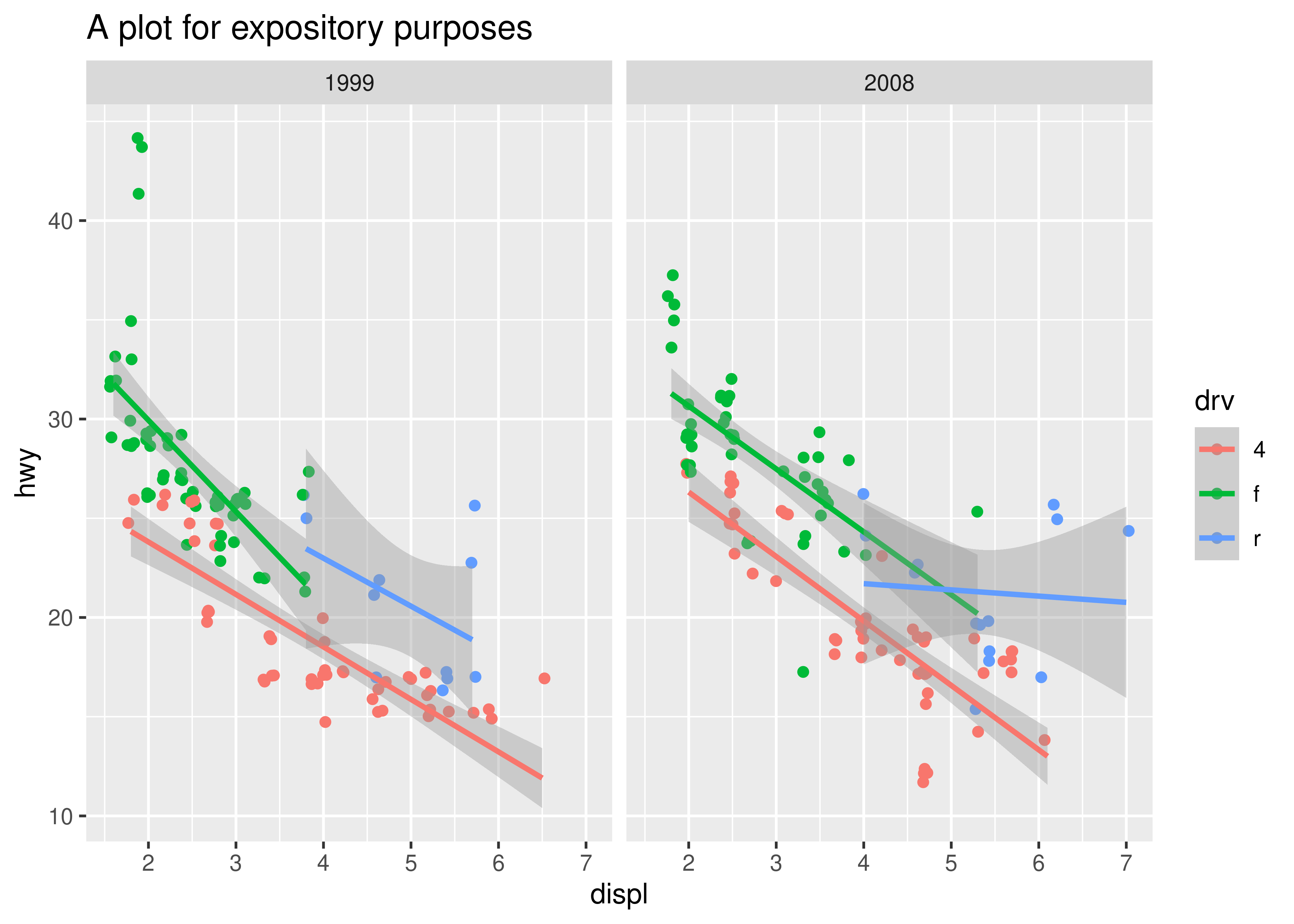
The code in our simplified print method reveals four distinct steps:
First, it calls
ggplot_build()where the data for each layer is prepared and organised into a standardised format suitable for plotting.Second, the prepared data is passed to the
ggplot_gtable()and turns it into graphic elements stored in a gtable (we’ll come back to what that is later).Third, the gtable object is converted to an image with the assistance of the grid package.
Fourth, the original ggplot object is invisibly returned to the user.
One thing that this process reveals is that ggplot2 itself does none of the low-level drawing: its responsibility ends when the gtable object has been created. Nor does the gtable package (which implements the gtable class) do any drawing. All drawing is performed by the grid package together with the active graphics device. This is an important point, as it means ggplot2 – or any extension to ggplot2 – does not concern itself with the nitty gritty of creating the visual output. Rather, its job is to convert user data to one or more graphical primitives such as polygons, lines, points, etc and then hand responsibility over to the grid package.
Although it is not strictly correct to do so, we will refer to this conversion into graphical primitives as the rendering process. The next two sections follow the data down the rendering rabbit hole through the build step (Section 19.2) and the gtable step (Section 19.3) whereupon – rather like Alice in Lewis Carroll’s novel – it finally arrives in the grid wonderland as a collection of graphical primitives.
19.2 The build step
ggplot_build(), as discussed above, takes the declarative representation constructed with the public API and augments it by preparing the data for conversion to graphic primitives.
19.2.1 Data preparation
The first part of the processing is to get the data associated with each layer and get it into a predictable format. A layer can either provide data in one of three ways: it can supply its own (e.g., if the data argument to a geom is a data frame), it can inherit the global data supplied to ggplot(), or else it might provide a function that returns a data frame when applied to the global data. In all three cases the result is a data frame that is passed to the plot layout, which orchestrates coordinate systems and facets. When this happens the data is first passed to the plot coordinate system which may change it (but usually doesn’t), and then to the facet which inspects the data to figure out how many panels the plot should have and how they should be organised. During this process the data associated with each layer will be augmented with a PANEL column. This column will (must) be kept throughout the rendering process and is used to link each data row to a specific facet panel in the final plot.
The last part of the data preparation is to convert the layer data into calculated aesthetic values. This involves evaluating all aesthetic expressions from aes() on the layer data. Further, if not given explicitly, the group aesthetic is calculated from the interaction of all non-continuous aesthetics. The group aesthetic is, like PANEL a special column that must be kept throughout the processing. As an example, the plot p created earlier contains only the one layer specified by geom_point() and at the end of the data preparation process the first 10 rows of the data associated with this layer look like this:
#>      x  y colour PANEL group
#> 1  1.8 29      f     1     2
#> 2  1.8 29      f     1     2
#> 3  2.0 31      f     2     2
#> 4  2.0 30      f     2     2
#> 5  2.8 26      f     1     2
#> 6  2.8 26      f     1     2
#> 7  3.1 27      f     2     2
#> 8  1.8 26      4     1     1
#> 9  1.8 25      4     1     1
#> 10 2.0 28      4     2     1
19.2.2 Data transformation
Once the layer data has been extracted and converted to a predictable format it undergoes a series of transformations until it has the format expected by the layer geometry.
The first step is to apply any scale transformations to the columns in the data. It is at this stage of the process that any argument to trans in a scale has an effect, and all subsequent rendering will take place in this transformed space. This is the reason why setting a position transform in the scale has a different effect than setting it in the coordinate system. If the transformation is specified in the scale it is applied before any other calculations, but if it is specified in the coordinate system the transformation is applied after those calculations. For instance, our original plot p involves no scale transformations so the layer data remain untouched at this stage. The first three rows are shown below:
#>     x  y colour PANEL group
#> 1 1.8 29      f     1     2
#> 2 1.8 29      f     1     2
#> 3 2.0 31      f     2     2
In contrast, if our plot object is p + scale_x_log10() and we inspect the layer data at this point in processing, we see that the x variable has been transformed appropriately:
#>       x  y colour PANEL group
#> 1 0.255 29      f     1     2
#> 2 0.255 29      f     1     2
#> 3 0.301 31      f     2     2
The second step in the process is to map the position aesthetics using the position scales, which unfolds differently depending on the kind of scale involved. For continuous position scales – such as those used in our example – the out of bounds function specified in the oob argument (Section 14.4) is applied at this point, and NA values in the layer data are removed. This makes little difference for p, but if we were plotting p + xlim(2, 8) instead the oob function – scales::censor() in this case – would replace x values below 2 with NA as illustrated below:
#> Warning: Removed 22 rows containing non-finite outside the scale range
#> (`stat_smooth()`).
#>    x  y colour PANEL group
#> 1 NA 29      f     1     2
#> 2 NA 29      f     1     2
#> 3  2 31      f     2     2
For discrete positions the change is more radical, because the values are matched to the limits values or the breaks specification provided by the user, and then converted to integer-valued positions. Finally, for binned position scales the continuous data is first cut into bins using the breaks argument, and the position for each bin is set to the midpoint of its range. The reason for performing the mapping at this stage of the process is consistency: no matter what type of position scale is used, it will look continuous to the stat and geom computations. This is important because otherwise computations such as dodging and jitter would fail for discrete scales.
At the third stage in this transformation the data is handed to the layer stat where any statistical transformation takes place. The procedure is as follows: first, the stat is allowed to inspect the data and modify its parameters, then do a one off preparation of the data. Next, the layer data is split by PANEL and group, and statistics are calculated before the data is reassembled.2 Once the data has been reassembled in its new form it goes through another aesthetic mapping process. This is where any aesthetics whose computation has been delayed using stat() (or the old ..var.. notation) get added to the data. Notice that this is why stat() expressions – including the formula used to specify the regression model in the geom_smooth() layer of our example plot p – cannot refer to the original data. It simply doesn’t exist at this point.
As an example consider the second layer in our plot, which produces the linear regressions. Before the stat computations have been performed the data for this layer simply contain the coordinates and the required PANEL and group columns.
#>     x  y colour PANEL group
#> 1 1.8 29      f     1     2
#> 2 1.8 29      f     1     2
#> 3 2.0 31      f     2     2
After the stat computations have taken place, the layer data are changed considerably:
#>      x    y ymin ymax    se flipped_aes colour PANEL group
#> 1 1.80 24.3 23.1 25.6 0.625       FALSE      4     1     1
#> 2 1.86 24.2 22.9 25.4 0.612       FALSE      4     1     1
#> 3 1.92 24.0 22.8 25.2 0.598       FALSE      4     1     1
At this point the geom takes over from the stat (almost). The first action it takes is to inspect the data, update its parameters and possibly make a first pass modification of the data (same setup as for stat). This is possibly where some of the columns gets reparameterised e.g. x+width gets changed to xmin+xmax. After this the position adjustment gets applied, so that e.g. overlapping bars are stacked, etc. For our example plot p, it is at this step that the jittering is applied in the first layer of the plot and the x and y coordinates are perturbed:
#>      x    y colour PANEL group
#> 1 1.84 28.8      f     1     2
#> 2 1.77 29.1      f     1     2
#> 3 2.83 26.0      f     1     2
Next—and perhaps surprisingly—the position scales are all reset, retrained, and applied to the layer data. Thinking about it, this is absolutely necessary because, for example, stacking can change the range of one of the axes dramatically. In some cases (e.g., in the histogram example above) one of the position aesthetics may not even be available until after the stat computations and if the scales were not retrained it would never get trained.
The last part of the data transformation is to train and map all non-positional aesthetics, i.e. convert whatever discrete or continuous input that is mapped to graphical parameters such as colours, linetypes, sizes etc. Further, any default aesthetics from the geom are added so that the data is now in a predictable state for the geom. At the very last step, both the stat and the facet gets a last chance to modify the data in its final mapped form with their finish_data() methods before the build step is done. For the plot object p, the first few rows from final state of the layer data look like this:
#>      x    y  colour PANEL group shape fill size alpha stroke
#> 1 1.83 29.3 #00BA38     1     2    19   NA  1.5    NA    0.5
#> 2 1.79 28.7 #00BA38     1     2    19   NA  1.5    NA    0.5
#> 3 2.79 26.3 #00BA38     1     2    19   NA  1.5    NA    0.5
19.2.3 Output
The return value of ggplot_build() is a list structure with the ggplot_built class. It contains the computed data, as well as a Layout object holding information about the trained coordinate system and faceting. Further it holds a copy of the original plot object, but now with trained scales.
19.3 The gtable step
The purpose of ggplot_gtable() is to take the output of the build step and, with the help of the gtable package, turn it into an object that can be plotted using grid (we’ll talk more about gtable in Section 21.5.6). At this point the main elements responsible for further computations are the geoms, the coordinate system, the facet, and the theme. The stats and position adjustments have all played their part already.
19.3.1 Rendering the panels
The first thing that happens is that the data is converted into its graphical representation. This happens in two steps. First, each layer is converted into a list of graphical objects (grobs). As with stats the conversion happens by splitting the data, first by PANEL, and then by group, with the possibility of the geom intercepting this splitting for performance reasons. While a lot of the data preparation has been performed already it is not uncommon that the geom does some additional transformation of the data during this step. A crucial part is to transform and normalise the position data. This is done by the coordinate system and while it often simply means that the data is normalised based on the limits of the coordinate system, it can also include radical transformations such as converting the positions into polar coordinates. The output of this is for each layer a list of gList objects corresponding to each panel in the facet layout. After this the facet takes over and assembles the panels. It does this by first collecting the grobs for each panel from the layers, along with rendering strips, backgrounds, gridlines, and axes based on the theme and combines all of this into a single gList for each panel. It then proceeds to arranging all these panels into a gtable based on the calculated panel layout. For most plots this is simple as there is only a single panel, but for e.g. plots using facet_wrap() it can be quite complicated. The output is the basis of the final gtable object. At this stage in the process our example plot p looks like this:
19.3.2 Adding guides
There are two types of guides in ggplot2: axes and legends. As our plot p illustrates at this point the axes have already been rendered and assembled together with the panels, but the legends are still missing. Rendering the legends is a complicated process that first trains a guide for each scale. Then, potentially multiple guides are merged if their mapping allows it, before the layers that contribute to the legend are asked for key grobs for each key in the legend. These key grobs are then assembled across layers and combined to the final legend in a process that is quite reminiscent of how layers are combined into the gtable of panels. In the end the output is a gtable that holds each legend box arranged and styled according to the theme and guide specifications. Once created the guide gtable is then added to the main gtable according to the legend.position theme setting. At this stage, our example plot is complete in most respects: the only thing missing is the title.
19.3.3 Adding adornment
The only thing remaining is to add title, subtitle, caption, and tag as well as add background and margins, at which point the final gtable is done.
19.3.4 Output
At this point ggplot2 is ready to hand over to grid. Our rendering process is more or less equivalent to the code below and the end result is, as described above, a gtable:
p_built <- ggplot_build(p)
p_gtable <- ggplot_gtable(p_built)

class(p_gtable)
#> [1] "gtable" "gTree"  "grob"   "gDesc"
What is less obvious is that the dimensions of the object are unpredictable and will depend on both the faceting, legend placement, and which titles are drawn. It is thus not advised to depend on row and column placement in your code, should you want to further modify the gtable. All elements of the gtable are named though, so it is still possible to reliably retrieve, e.g. the grob holding the top-left y-axis with a bit of work. As an illustration, the gtable for our plot p is shown in the code below:
p_gtable
#> TableGrob (17 x 17) "layout": 25 grobs
#> z cells name
#> 1 0 ( 1-17, 1-17) background
#> 2 1 (10-10, 7- 7) panel-1-1
#> 3 1 (10-10,11-11) panel-2-1
#> 4 3 ( 8- 8, 7- 7) axis-t-1-1
#> 5 3 ( 8- 8,11-11) axis-t-2-1
#> 6 3 (11-11, 7- 7) axis-b-1-1
#> 7 3 (11-11,11-11) axis-b-2-1
#> 8 3 (10-10,10-10) axis-l-1-2
#> 9 3 (10-10, 6- 6) axis-l-1-1
#> 10 3 (10-10,12-12) axis-r-1-2
#> 11 3 (10-10, 8- 8) axis-r-1-1
#> 12 2 ( 9- 9, 7- 7) strip-t-1-1
#> 13 2 ( 9- 9,11-11) strip-t-2-1
#> 14 4 ( 7- 7, 7-11) xlab-t
#> 15 5 (12-12, 7-11) xlab-b
#> 16 6 (10-10, 5- 5) ylab-l
#> 17 7 (10-10,13-13) ylab-r
#> 18 8 (10-10,15-15) guide-box-right
#> 19 9 (10-10, 3- 3) guide-box-left
#> 20 10 (14-14, 7-11) guide-box-bottom
#> 21 11 ( 5- 5, 7-11) guide-box-top
#> 22 12 (10-10, 7-11) guide-box-inside
#> 23 13 ( 4- 4, 7-11) subtitle
#> 24 14 ( 3- 3, 7-11) title
#> 25 15 (15-15, 7-11) caption
#> grob
#> 1 rect[plot.background..rect.719]
#> 2 gTree[panel-1.gTree.596]
#> 3 gTree[panel-2.gTree.611]
#> 4 zeroGrob[NULL]
#> 5 zeroGrob[NULL]
#> 6 absoluteGrob[GRID.absoluteGrob.615]
#> 7 absoluteGrob[GRID.absoluteGrob.615]
#> 8 zeroGrob[NULL]
#> 9 absoluteGrob[GRID.absoluteGrob.623]
#> 10 zeroGrob[NULL]
#> 11 zeroGrob[NULL]
#> 12 gtable[strip]
#> 13 gtable[strip]
#> 14 zeroGrob[NULL]
#> 15 titleGrob[axis.title.x.bottom..titleGrob.678]
#> 16 titleGrob[axis.title.y.left..titleGrob.681]
#> 17 zeroGrob[NULL]
#> 18 gtable[guide-box]
#> 19 zeroGrob[NULL]
#> 20 zeroGrob[NULL]
#> 21 zeroGrob[NULL]
#> 22 zeroGrob[NULL]
#> 23 zeroGrob[plot.subtitle..zeroGrob.716]
#> 24 titleGrob[plot.title..titleGrob.715]
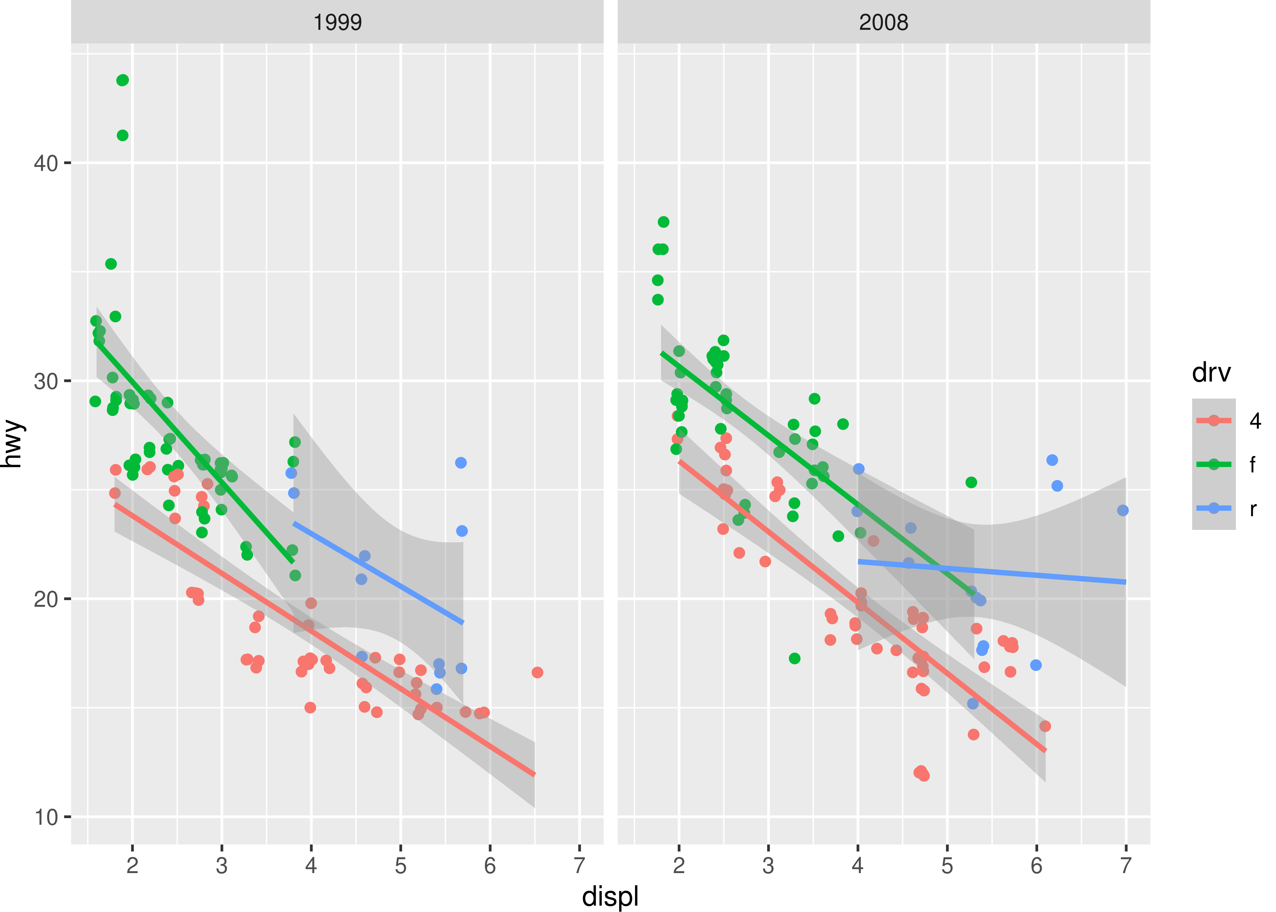
#> 25 zeroGrob[plot.caption..zeroGrob.717]The final plot, as one would hope, looks identical to the original:
grid::grid.newpage()
grid::grid.draw(p_gtable)
19.4 Introducing ggproto
Section 19.1 to Section 19.3 focus on the sequence of events involved in building a ggplot, but are intentionally vague as to what kind of programming objects perform this work.
All ggplot2 objects are built using the ggproto system for object-oriented programming, and is unusual in that it is used only by ggplot2. This is something of a historical accident: ggplot2 originally used proto (Grothendieck et al. 2016) for object-oriented programming, which became a problem once the need for an official extension mechanism arose due to the limitations of the proto system. Attempts to switch ggplot2 to other systems such as R6 (Chang 2020) proved difficult, and creating an object-oriented system specific to the needs of ggplot2 turned out to be the least bad solution.
Understanding the ggproto object-oriented programming system is important if you wish to write ggplot2 extensions. We will encounter ggproto objects as they are used by ggplot2 in Chapter 20 and Chapter 21. Like the better-known R6 system, ggproto uses reference semantics and allows inheritance and access to methods from parent classes. It is accompanied by a set of design principles that, while not enforced by ggproto, is essential to understanding how the system is used in ggplot2. To illustrate these concepts, this section introduces the core mechanics of ggproto in a simplified form.
19.4.1 ggproto objects
Creating a new ggproto object is done with the ggproto() function, which takes the name of the new class as its first argument, and another ggproto object from which the new one will inherit from as the second argument. For example, we could create a ggproto object—albeit one that has no useful functionality—with the following command:
NewObject <- ggproto(
  `_class` = NULL,
  `_inherits` = NULL
)
By convention, ggproto objects are named using “UpperCamelCase”, in which each word begins with a capital letter. It is also conventional to omit the names of the `_class` and `_inherits` arguments, so the conventional form of this command would be as follows:
NewObject <- ggproto(NULL, NULL)If we print this object we see that it is indeed a ggproto object, but no other information appears.
NewObject
#> <ggproto object: Class gg>
19.4.2 Creating new classes
To create a new ggproto class, the only thing that is strictly necessary is to supply a class name as the first argument to ggproto(). A minimal command that defines a new class might look like this:
NewClass <- ggproto("NewClass", NULL)The NewClass variable still refers to a ggproto object, but we can verify that it has the desired class name by printing it:
NewClass
#> <ggproto object: Class NewClass, gg>
However, so far the only thing we have done is create an object that specifies a class. The NewClass object doesn’t do anything. To create a ggproto class that does something useful, we need to supply a list of fields and methods when we define the class. In this context, “fields” are used to store data relevant to the object, and “methods” are functions that can use the data stored in the object. Fields and methods are constructed in the same way, and they are not treated differently from a user perspective.
To illustrate this, we’ll create a new class called Person that will be used to store and manipulate information about a person. We can do this by supplying the ggproto() function with name/value pairs:
Person <- ggproto("Person", NULL,

  # fields
  given_name = NA,
  family_name = NA,
  birth_date = NA,

  # methods
  full_name = function(self, family_last = TRUE) {
    if(family_last == TRUE) {
      return(paste(self$given_name, self$family_name))
    }
    return(paste(self$family_name, self$given_name))
  },
  age = function(self) {
    days_old <- Sys.Date() - self$birth_date
    floor(as.integer(days_old) / 365.25)
  },
  description = function(self) {
    paste(self$full_name(), "is", self$age(), "years old")
  }
)
The Person class is now associated with three fields, corresponding to given_name and family_name of a person as well as their birth_date. It also possesses three methods: the full_name() method is a function that constructs the full name of the person, using the convention of placing the given name first and the family name second, the age() method calculates the age of the person in years, and the description() method prints out a short description of the person.
Printing the object shows the fields and methods with which it is associated:
Person
#> <ggproto object: Class Person, gg>
#>     age: function
#>     birth_date: NA
#>     description: function
#>     family_name: NA
#>     full_name: function
#>     given_name: NA
The Person ggproto object is essentially a template for the class, and we can use to create specific records of individual people (discussed in Section 19.4.3). If you are familiar with other object-oriented programming systems you might have been expecting something a little different: often new classes are defined with a dedicated constructor function. One quirk of ggproto is that ggproto() doesn’t do this: rather, the class constructor is itself an object.
Another thing to note when defining methods is the use of self as their first argument. This is a special argument used to give the method access to the fields and methods associated with the ggproto object (see Section 19.4.4 for an example). The special status of this argument is evident when printing a ggproto method:
Person$full_name
#> <ggproto method>
#>   <Wrapper function>
#>     function (...)
#> full_name(..., self = self)
#>
#>   <Inner function (f)>
#>     function (self, family_last = TRUE)
#> {
#>     if (family_last == TRUE) {
#>         return(paste(self$given_name, self$family_name))
#>     }
#>     return(paste(self$family_name, self$given_name))
#> }
This output may seem a little surprising: when we defined full_name() earlier we only provided the code listed as the “inner function”. What has happened is that ggproto() automatically enclosed my function within a wrapper function that calls my code as the inner function, while ensuring that an appropriate definition of self is used. When the method is printed, the console displays both the wrapper function (typically of little interest) and the inner function. Output in this format appears in Chapter 20 and Chapter 21.
19.4.3 Creating new instances
Now that we have defined the Person class, we can create instances of the class. This is done by passing a ggproto object as the second argument to ggproto(), and not specifying a new class name in the first argument. For instance, we can create new objects Thomas and Danielle that are both instances of the Person class as follows:
Specifying NULL as the first argument instructs ggproto() not to define a new class, but instead create a new instance of the class specified in the second argument. Because Thomas and Danielle are both instances of the Person class, they automatically inherit its age(), full_name() and description() methods:
Thomas$description()
#> [1] "Thomas Lin Pedersen is 40 years old"

Danielle$description()
#> [1] "Danielle Jasmine Navarro is 48 years old"
19.4.4 Creating subclasses
In the previous example we created Person as an entirely new class. In practice you will almost never need to do this: instead, you will likely be creating a subclass using an existing ggproto object. You can do this by specifying the name of the subclass and the object from which it should inherit in the call to ggproto():
# define the subclass
NewSubClass <- ggproto("NewSubClass", Person)

# verify that this works
NewSubClass
#> <ggproto object: Class NewSubClass, Person, gg>
#>     age: function
#>     birth_date: NA
#>     description: function
#>     family_name: NA
#>     full_name: function
#>     given_name: NA
#>     super:  <ggproto object: Class Person, gg>
The output shown above illustrates that NewSubClass now provides its own class, and that it inherits all the fields and methods from the Person object we created earlier. However, this new subclass does not add any new functionality.
When creating a subclass, we often want to add new fields or methods and overwrite some of the existing ones. For example, suppose we want to define Royalty as a subclass of Person, and add fields corresponding to the rank of the royal in question, and the territory over which they ruled. Because royalty are often referred to by title and territory rather than in terms of a first and last name, we will also need to change the way that the full_name() method is defined:
Royalty <- ggproto("Royalty", Person,
  rank = NA,
  territory = NA,
  full_name = function(self) {
    paste(self$rank, self$given_name, "of", self$territory)
  }
)
The Royalty object now defines a subclass of person that inherits some fields (given_name, family_name, birth_date) from the Person class, and supplies other fields (rank, territory). It inherits the age() and description() methods from Person, but it overwrites the full_name() method.
We can now create a new instance of the Royalty subclass:
Victoria <- ggproto(NULL, Royalty,
  given_name = "Victoria",
  family_name = "Hanover",
  rank = "Queen",
  territory = "the United Kingdom",
  birth_date = as.Date("1819/05/24")
)
So when we call the full_name() method for Victoria, the output uses the method specified in the Royalty class instead of the one defined in the Person class:
Victoria$full_name()
#> [1] "Queen Victoria of the United Kingdom"
It is worth noting what happens when we call the description() method. This method is inherited from Person, but the definition of this method invokes self$full_name(). Even though description() is defined in Person, in this context self still refers to Victoria, who is still Royalty. What this means is that the output of the inherited description() method uses the full_name() method defined for the subclass:
Victoria$description()
#> [1] "Queen Victoria of the United Kingdom is 207 years old"
Creating subclasses sometimes requires us to access the parent class and its methods, which we can do with the help of the ggproto_parent() function. For example we can define a Police subclass that includes a rank field in the same way that the Royalty subclass does, but only uses this rank as part of the description() method:
Police <- ggproto("Police", Person,
  rank = NA,
  description = function(self) {
    paste(
      self$rank,
      ggproto_parent(Person, self)$description()
    )
  }
)
In this example, the description() method for the Police subclass is defined in a way that explicitly refers to the description() method for the Person parent class. By using ggproto_parent(Person, self) in this fashion, we are able to refer to the method inside the parent class, while still retaining the appropriate local definition of self. As before, we’ll create a specific instance and verify that this works as expected:
John <- ggproto(NULL, Police,
  given_name = "John",
  family_name = "McClane",
  rank = "Detective",
  birth_date = as.Date("1955/03/19")
)

John$full_name()
#> [1] "John McClane"

John$description()
#> [1] "Detective John McClane is 71 years old"
For reasons that we’ll discuss below, the use of ggproto_parent() is not that prevalent in the ggplot2 source code.
19.4.5 Style guide for ggproto
Because ggproto is a minimal class system designed to accommodate ggplot2 and nothing else, it important to recognise that ggproto is used in ggplot2 in a very specific way. It exists to support the ggplot2 extension system, and you are unlikely to encounter ggproto in any context other than writing ggplot2 extension. With that in mind it is useful to understand how ggplot2 uses ggproto:
ggproto classes are used selectively. The use of ggproto in ggplot2 is not all-encompassing. Only select functionality is based on ggproto and it is neither expected nor advised to create entirely new ggproto classes in your extensions. As an extension developer, you will never create entirely ggproto objects but rather subclass one of the main ggproto classes provided by ggplot2. Chapter 20 and Chapter 21 will go into detail on how to do this.
ggproto classes are stateless. Except for a few internal classes that are used to orchestrate the rendering, ggproto classes in ggplot2 are assumed to be “stateless”. What this means is ggplot2 expects that after they are constructed, they will not change. This breaks a common expectation for reference-based classes (where methods often can safely change the state of the object), but it is not safe to do so with ggplot2. If your code violates this principle and changes the state of a Stat or Geom during the rendering, plotting a saved ggplot object will affect all instances of that Stat or Geom (even those used in other plots) because they all point to the same ggproto parent object. With this in mind, there are only two occasions when you should specify the state of a ggproto object in ggplot2. First, you can specify the state when creating the object: this is okay because this state should be shared between all instances anyway. Second, you can specify state via a params object managed elsewhere. As you’ll see later (see Section 20.2 and Section 20.3), most ggproto classes have a
setup_params()method where data can be inspected and specific properties calculated and stored.-
ggproto classes have simple inheritance. Because ggproto class instances are stateless, it is relatively safe to call methods that are defined inside other classes, instead of inheriting explicitly from the class. This is the reason why the
ggproto_parent()function is rarely called within the ggplot2 source code. As an example, thesetup_params()method inGeomErrorbaris defined as:GeomErrorbar <- ggproto( # ... setup_params = function(data, params) { GeomLinerange$setup_params(data, params) } # ... )This pattern is often easier to read than using
ggproto_parent()and because ggproto objects are stateless it is just as safe.
Chang, Winston. 2020. R6: Encapsulated Classes with Reference Semantics. https://CRAN.R-project.org/package=R6.
Grothendieck, Gabor, Louis Kates, and Thomas Petzoldt. 2016. Proto: Prototype Object-Based Programming. https://CRAN.R-project.org/package=proto.