14 Scales and guides

You are reading the work-in-progress third edition of the ggplot2 book. This chapter is currently a dumping ground for ideas, and we don’t recommend reading it.

The scales toolbox in Chapter 10 to Chapter 12 provides extensive guidance for how to work with scales, focusing on solving common data visualisation problems. The practical goals of the toolbox mean that topics are introduced when they are most relevant: for example, scale transformations are discussed in relation to continuous position scales (Section 10.1.7) because that is the most common situation in which you might want to transform a scale. However, because ggplot2 aims to provide a grammar of graphics, there is nothing preventing you from transforming other kinds of scales (see Section 14.6). This chapter aims to illustrate these concepts: We’ll discuss the theory underpinning scales and guides, and give examples showing how concepts that we’ve discussed specifically for position or colour scales also apply elsewhere.

14.1 Theory of scales and guides

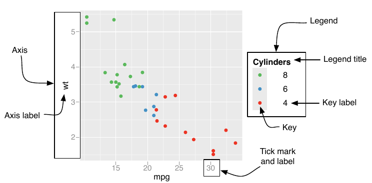
Formally, each scale is a function from a region in data space (the domain of the scale) to a region in aesthetic space (the range of the scale). The axis or legend is the inverse function, known as the guide: it allows you to convert visual properties back to data. You might find it surprising that axes and legends are the same type of thing, but while they look very different, they have the same purpose: to allow you to read observations from the plot and map them back to their original values. The commonalities between the two are illustrated below:

Argument name	Axis	Legend
`name`	Label	Title
`breaks`	Ticks & grid line	Key
`labels`	Tick label	Key label

However, legends are more complicated than axes, and consequently there are a number of topics that are specific to legends:

A legend can display multiple aesthetics (e.g. colour and shape), from multiple layers (Section 14.7.1), and the symbol displayed in a legend varies based on the geom used in the layer (Section 14.8)
Axes always appear in the same place. Legends can appear in different places, so you need some global way of positioning them.
Legends have more details that can be tweaked: should they be displayed vertically or horizontally? How many columns? How big should the keys be? This is discussed in (Section 14.5)

14.1.1 Scale specification

An important property of ggplot2 is the principle that every aesthetic in your plot is associated with exactly one scale. For instance, when you write this

ggplot(mpg, aes(displ, hwy)) + 
  geom_point(aes(colour = class))

ggplot2 adds a default scale for each aesthetic used in the plot:

ggplot(mpg, aes(displ, hwy)) + 
  geom_point(aes(colour = class)) +
  scale_x_continuous() + 
  scale_y_continuous() + 
  scale_colour_discrete()

The choice of default scale depends on the aesthetic and the variable type. In this example hwy is a continuous variable mapped to the y aesthetic so the default scale is scale_y_continuous(); similarly class is discrete so when mapped to the colour aesthetic the default scale becomes scale_colour_discrete(). Specifying these defaults would be tedious so ggplot2 does it for you. But if you want to override the defaults, you’ll need to add the scale yourself, like this:

ggplot(mpg, aes(displ, hwy)) + 
  geom_point(aes(colour = class)) + 
  scale_x_continuous(name = "A really awesome x axis label") +
  scale_y_continuous(name = "An amazingly great y axis label")

In practice you would typically use labs() for this, discussed in Section 8.1, but it is conceptually helpful to understand that axis labels and legend titles are both examples of scale names: see Section 14.2.

The use of + to “add” scales to a plot is a little misleading because if you supply two scales for the same aesthetic, the last scale takes precedence. In other words, when you + a scale, you’re not actually adding it to the plot, but overriding the existing scale. This means that the following two specifications are equivalent:

ggplot(mpg, aes(displ, hwy)) + 
  geom_point() + 
  scale_x_continuous(name = "Label 1") +
  scale_x_continuous(name = "Label 2")
#> Scale for x is already present.
#> Adding another scale for x, which will replace the existing scale.

ggplot(mpg, aes(displ, hwy)) + 
  geom_point() + 
  scale_x_continuous(name = "Label 2")

Note the message when you add multiple scales for the same aesthetic, which makes it harder to accidentally overwrite an existing scale. If you see this in your own code, you should make sure that you’re only adding one scale to each aesthetic.

If you’re making small tweaks to the scales, you might continue to use the default scales, supplying a few extra arguments. If you want to make more radical changes you will override the default scales with alternatives:

ggplot(mpg, aes(displ, hwy)) + 
  geom_point(aes(colour = class)) +
  scale_x_sqrt() + 
  scale_colour_brewer()

Here scale_x_sqrt() changes the scale for the x axis scale, and scale_colour_brewer() does the same for the colour scale.

14.1.2 Naming scheme

The scale functions intended for users all follow a common naming scheme. You’ve probably already figured out the scheme, but to be concrete, it’s made up of three pieces separated by “_”:

scale
The name of the primary aesthetic (e.g., colour, shape or x)
The name of the scale (e.g., continuous, discrete, brewer).

The naming structure is often helpful, but can sometimes be ambiguous. For example, it is immediately clear that scale_x_*() functions apply to the x aesthetic, but it takes a little more thought to recognise that they also govern the behaviour of other aesthetics that describe a horizontal position (e.g., the xmin, xmax, and xend aesthetics). Similarly, while the name scale_colour_continuous() clearly refers to the colour scale associated with a continuous variables, it is less obvious that scale_colour_distiller() is simply a different method for creating colour scales for continuous variables.

14.1.3 Fundamental scale types

It is useful to note that internally all scale functions in ggplot2 belong to one of three fundamental types; continuous scales, discrete scales, and binned scales. Each fundamental type is handled by one of three scale constructor functions; continuous_scale(), discrete_scale() and binned_scale(). Although you should never need to call these constructor functions, they provide the organising structure for scales and it is useful to know about them.

14.2 Scale names

Extend discussion of labs() in Section 8.1.

14.3 Scale breaks

Discussion of what unifies the concept of breaks across continuous, discrete and binned scales: they are specific data values at which the guide needs to display something. Include additional detail about break functions.

14.4 Scale limits

Section 14.1 introduced the concept that a scale defines a mapping from the data space to the aesthetic space. Scale limits are an extension of this idea: they dictate the region of the data space over which the mapping is defined. At a theoretical level this region is defined differently depending on the fundamental scale type. For continuous and binned scales, the data space is inherently continuous and one-dimensional, so the limits can be specified by two end points. For discrete scales, however, the data space is unstructured and consists only of a set of categories: as such the limits for a discrete scale can only be specified by enumerating the set of categories over which the mapping is defined.

The toolbox chapters outline the common practical goals for specifying the limits: for position scales the limits are used to set the end points of the axis, for example. This leads naturally to the question of what ggplot2 should do if the data set contains “out of bounds” values that fall outside the limits.

The default behaviour in ggplot2 is to convert out of bounds values to NA, the logic for this being that if a data value is not part of the mapped region, it should be treated as missing. This can occasionally lead to unexpected behaviour, as illustrated in Section 10.1.2. You can override this default by setting oob argument of the scale, a function that is applied to all observations outside the scale limits. The default is scales::oob_censor() which replaces any value outside the limits with NA. Another option is scales::oob_squish() which squishes all values into the range. An example using a fill scale is shown below:

df <- data.frame(x = 1:6, y = 8:13)
base <- ggplot(df, aes(x, y)) + 
  geom_col(aes(fill = x)) +                    # bar chart
  geom_vline(xintercept = 3.5, colour = "red") # for visual clarity only

base
base + scale_fill_gradient(limits = c(1, 3))
base + scale_fill_gradient(limits = c(1, 3), oob = scales::squish)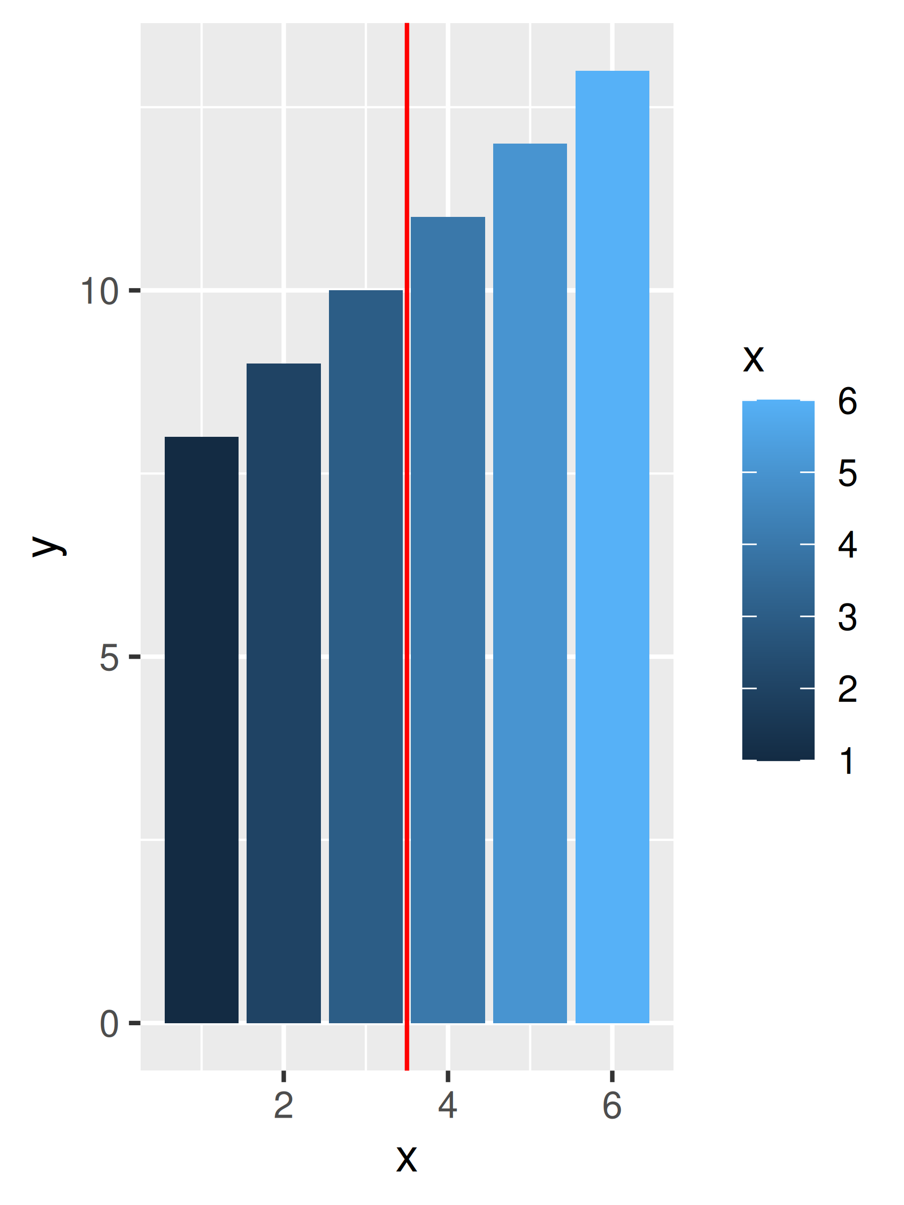

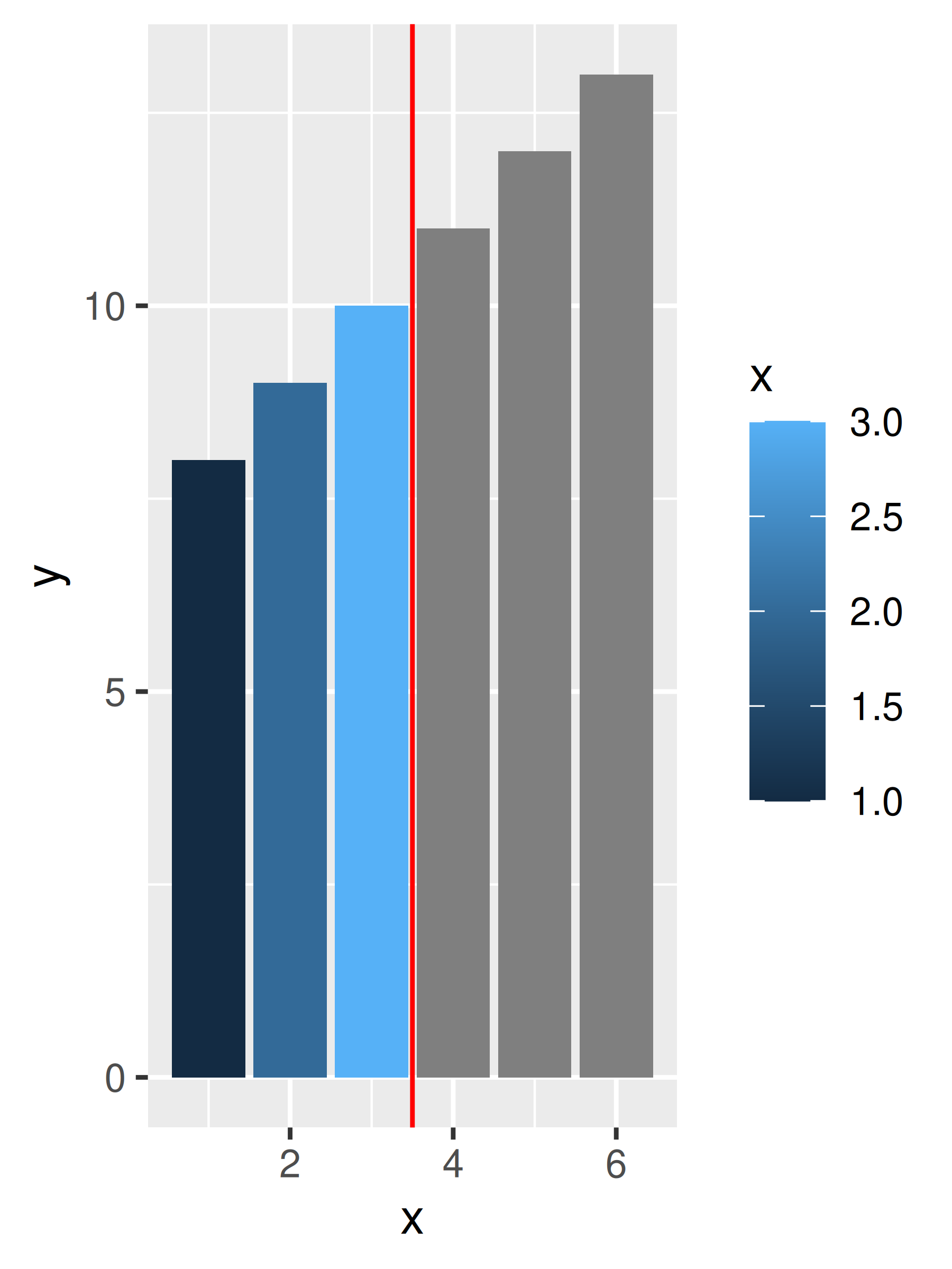
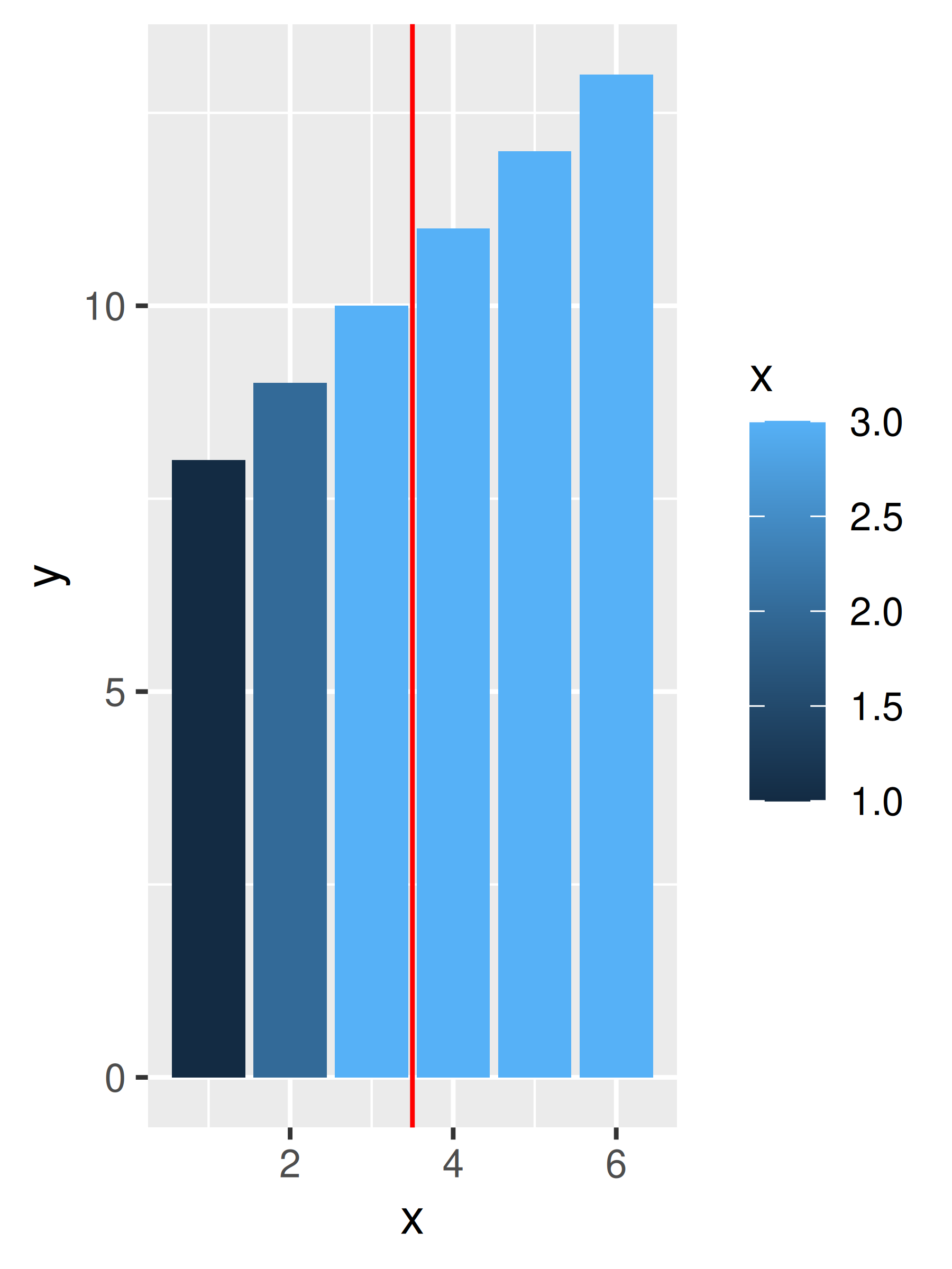
On the left the default fill colours are shown, ranging from dark blue to light blue. In the middle panel the scale limits for the fill aesthetic are reduced so that the values for the three rightmost bars are replace with NA and are mapped to a grey shade. In some cases, this is desired behaviour but often it is not: the right panel addresses this by modifying the oob function appropriately.

14.5 Scale guides

Scale guides are more complex than scale names: where the name argument (and labs() ) takes text as input, the guide argument (and guides()) require a guide object created by a guide function such as guide_colourbar() and guide_legend(). These arguments to these functions offer additional fine control over the guide.

The table below summarises the default guide functions associated with different scale types:

Scale type	Default guide type
continuous scales for colour/fill aesthetics	colourbar
binned scales for colour/fill aesthetics	coloursteps
position scales (continuous, binned and discrete)	axis
discrete scales (except position scales)	legend
binned scales (except position/colour/fill scales)	bins

Each of these guide types has appeared earlier in the toolbox:

guide_colourbar() is discussed in Section 11.2.5
guide_coloursteps() is discussed in Section 11.4.2
guide_axis() is discussed in Section 10.3.2
guide_legend() is discussed in Section 11.3.6
guide_bins() is discussed in Section 12.1.2

In addition to the functionality discussed in those sections, the guide functions have many arguments that are equivalent to theme settings like text colour, size, font etc, but only apply to a single guide. For information about those settings, see Chapter 17.

New stuff: show examples where something other than the default guide is used…

14.6 Scale transformation

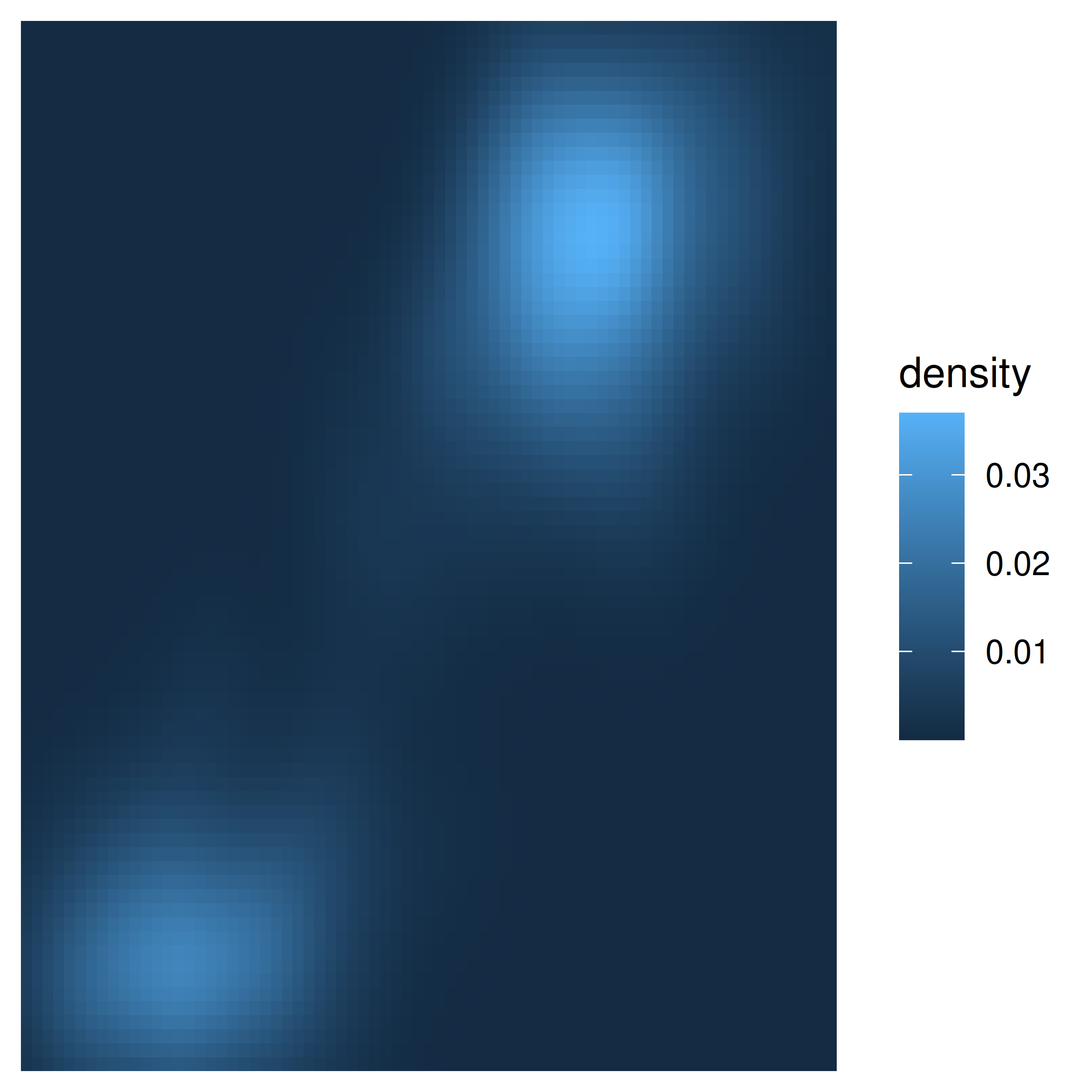
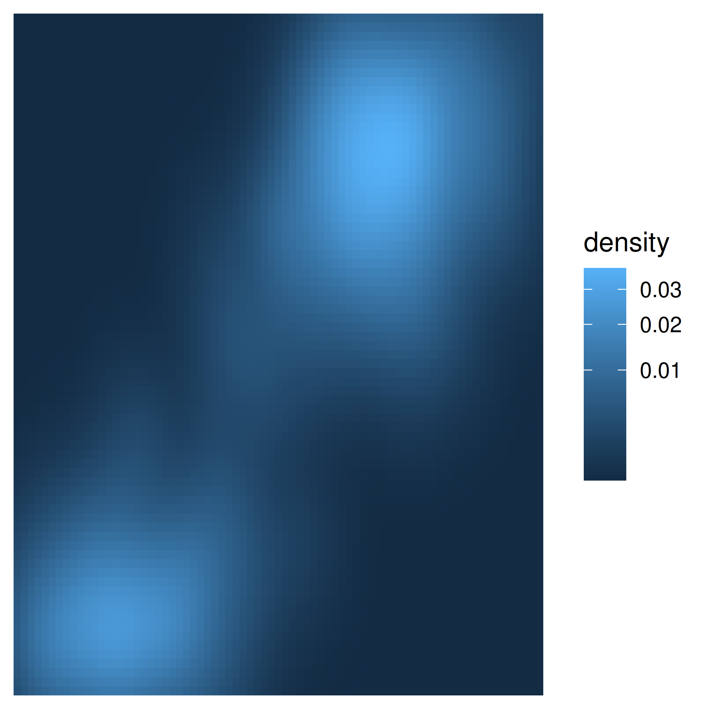
The most common use for scale transformations is to adjust a continuous position scale, as discussed in Section 10.1.7. However, they can sometimes be helpful to when applied to other aesthetics. Often this is purely a matter of visual emphasis. An example of this for the Old Faithful density plot is shown below. The linearly mapped scale on the left makes it easy to see the peaks of the distribution, whereas the transformed representation on the right makes it easier to see the regions of non-negligible density around those peaks:

base <- ggplot(faithfuld, aes(waiting, eruptions)) + 
  geom_raster(aes(fill = density)) + 
  scale_x_continuous(NULL, NULL, expand = c(0, 0)) +
  scale_y_continuous(NULL, NULL, expand = c(0, 0))
  
base
base + scale_fill_continuous(trans = "sqrt")

Transforming size aesthetics is also possible:

df <- data.frame(x = runif(20), y = runif(20), z = sample(20))
base <- ggplot(df, aes(x, y, size = z)) + geom_point()

base 
base + scale_size(trans = "reverse")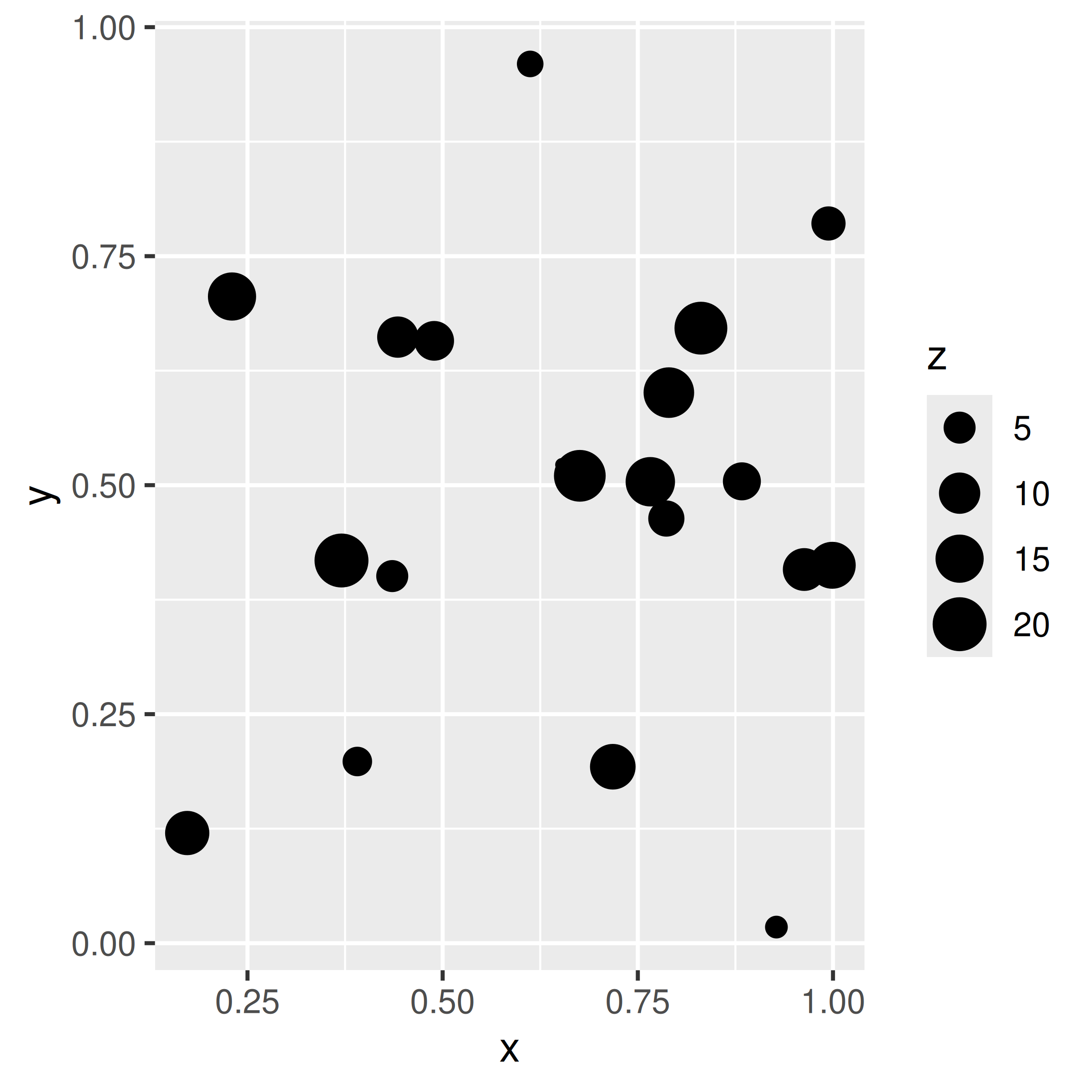

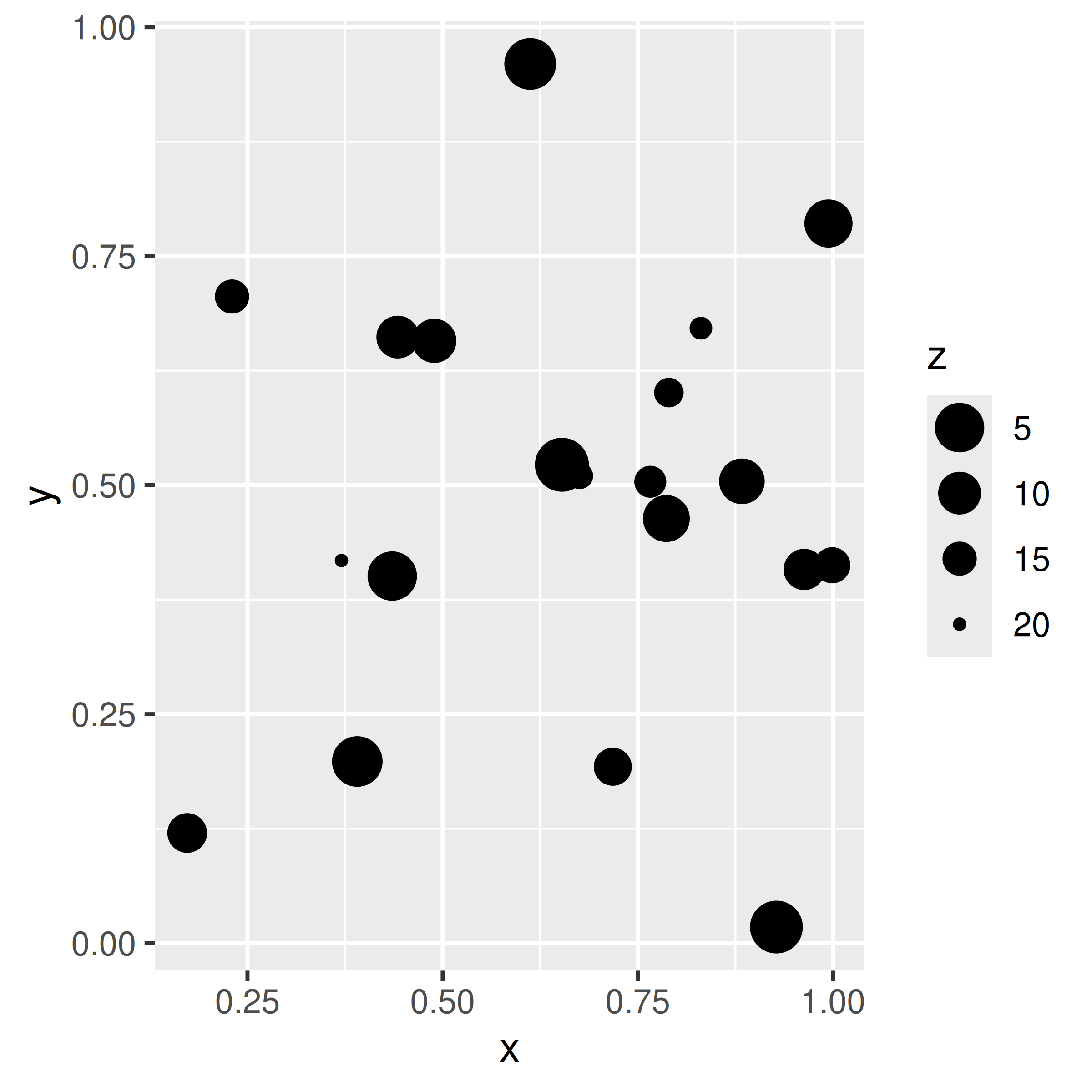
In the plot on the left, the z value is naturally interpreted as a “weight”: if each dot corresponds to a group, the z value might be the size of the group. In the plot on the right, the size scale is reversed, and z is more naturally interpreted as a “distance” measure: distant entities are scaled to appear smaller in the plot.

14.7 Legend merging and splitting

There is always a one-to-one correspondence between position scales and axes. But the connection between non-position scales and legend is more complex: one legend may need to draw symbols from multiple layers (“merging”), or one aesthetic may need multiple legends (“splitting”).

14.7.1 Merging legends

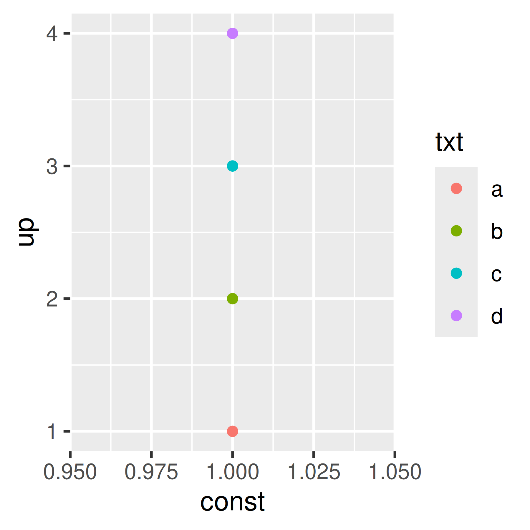
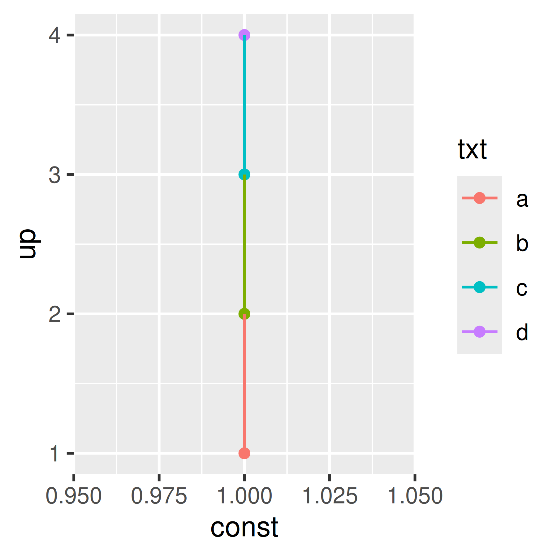
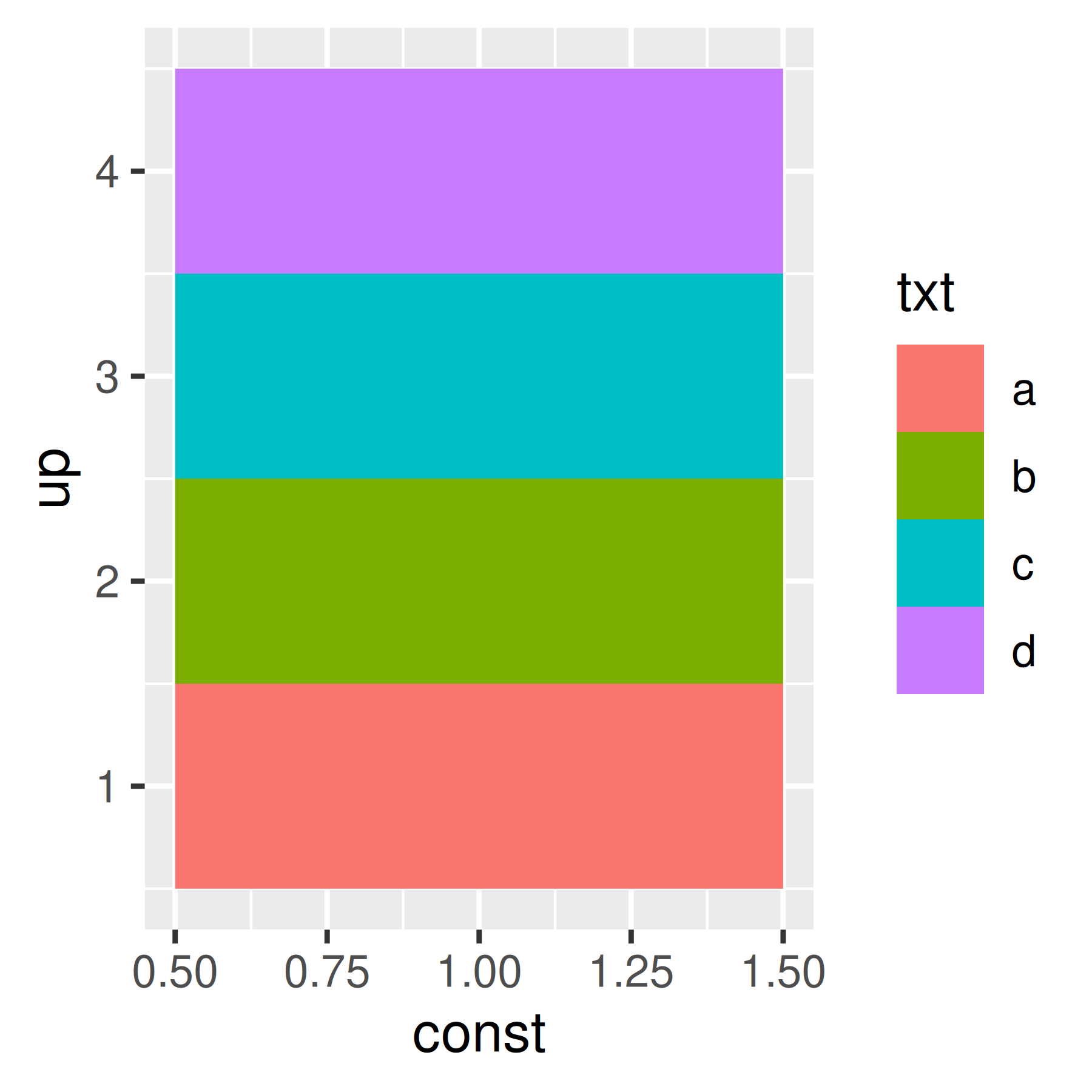
Merging legends occurs quite frequently when using ggplot2. For example, if you’ve mapped colour to both points and lines, the keys will show both points and lines. If you’ve mapped fill colour, you get a rectangle. Note the way the legend varies in the plots below:

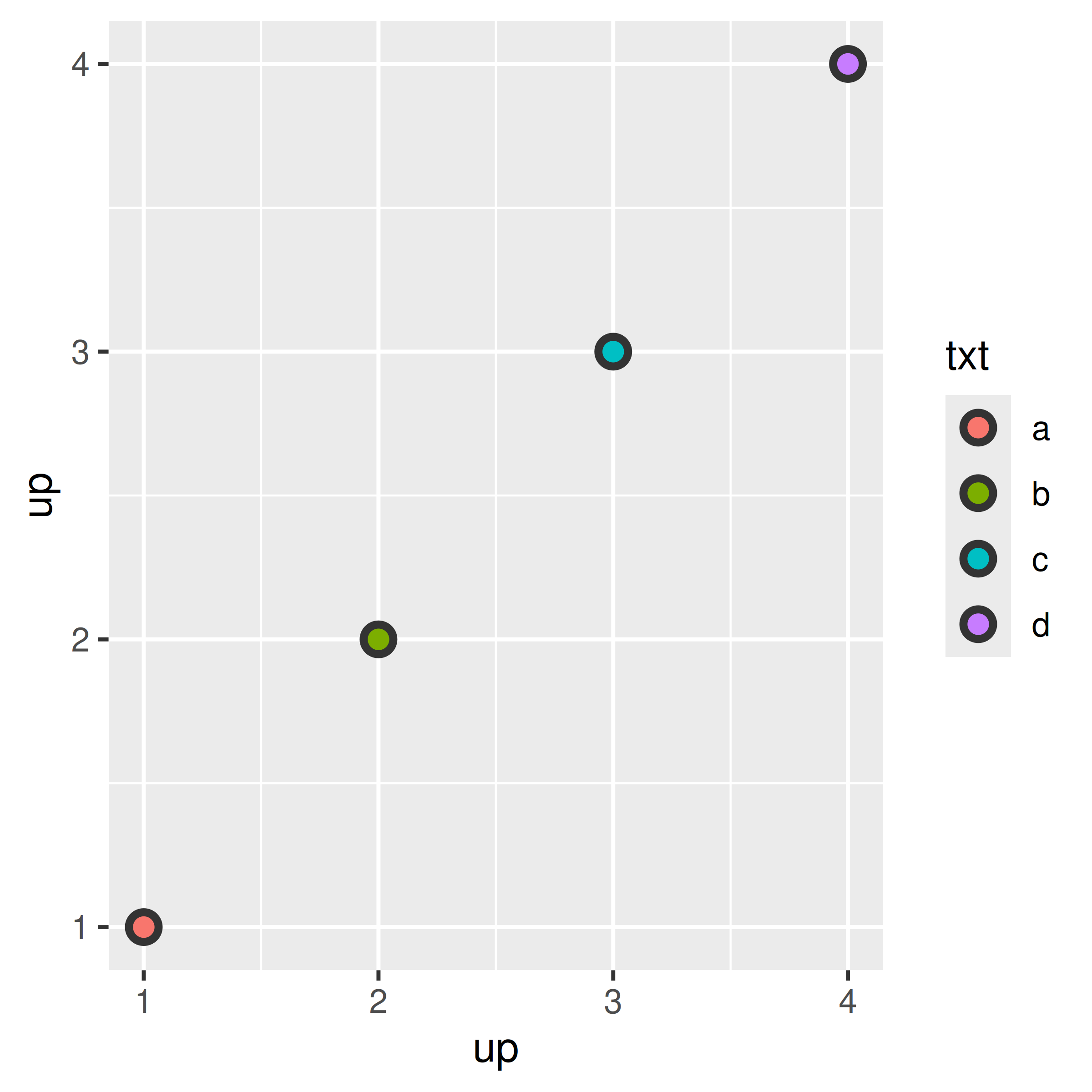
By default, a layer will only appear if the corresponding aesthetic is mapped to a variable with aes(). You can override whether or not a layer appears in the legend with show.legend: FALSE to prevent a layer from ever appearing in the legend; TRUE forces it to appear when it otherwise wouldn’t. Using TRUE can be useful in conjunction with the following trick to make points stand out:

ggplot(toy, aes(up, up)) + 
  geom_point(size = 4, colour = "grey20") +
  geom_point(aes(colour = txt), size = 2) 

ggplot(toy, aes(up, up)) + 
  geom_point(size = 4, colour = "grey20", show.legend = TRUE) +
  geom_point(aes(colour = txt), size = 2)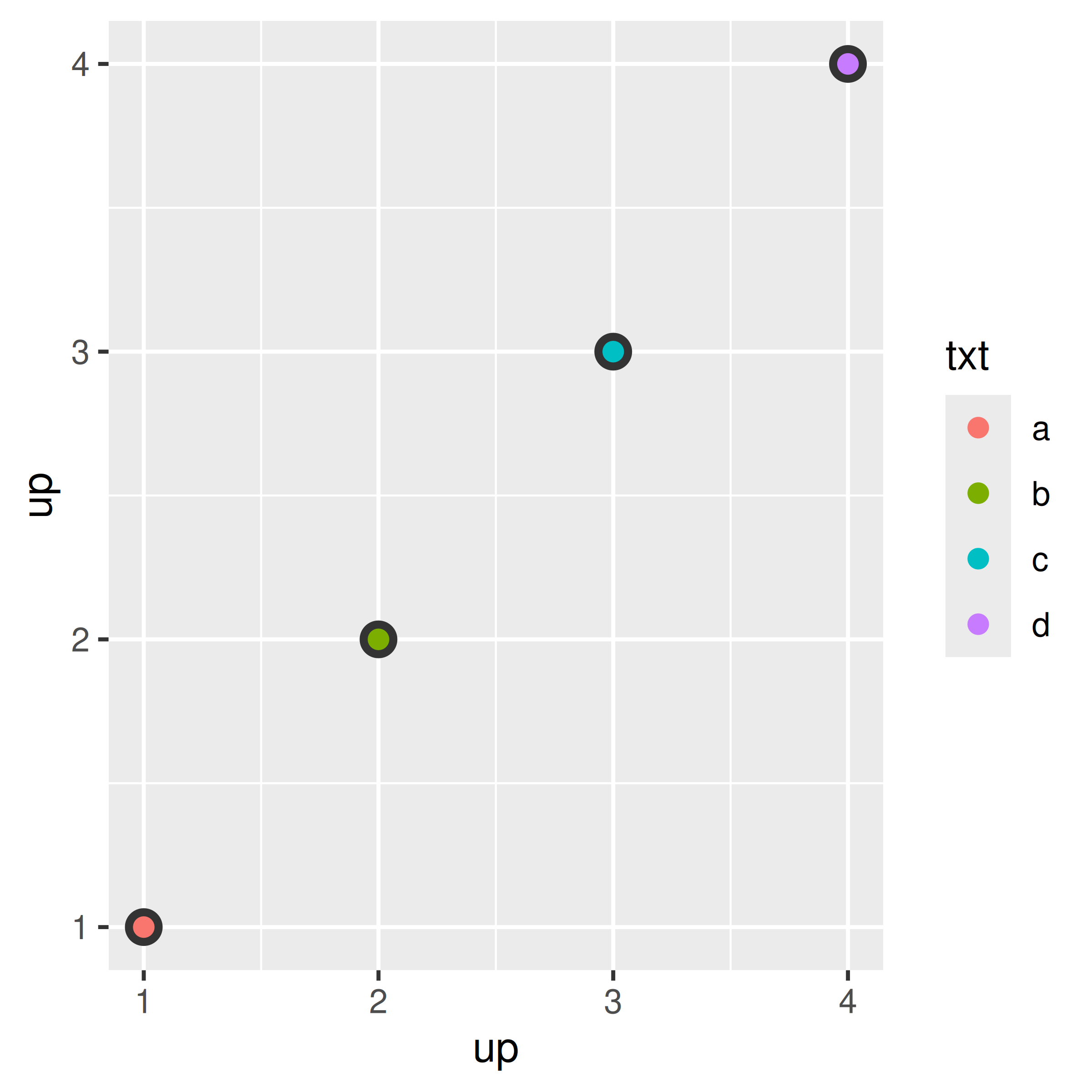

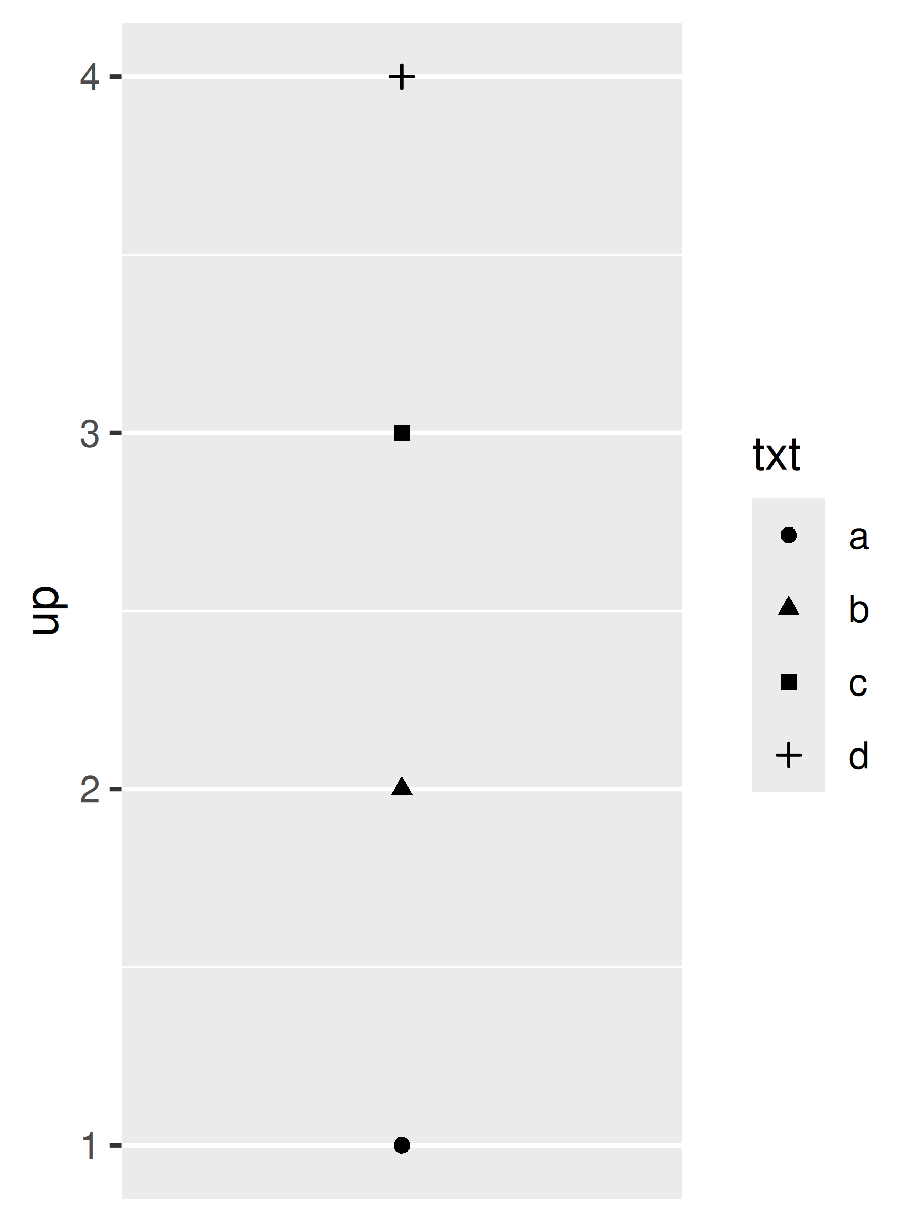
ggplot2 tries to use the fewest number of legends to accurately convey the aesthetics used in the plot. It does this by combining legends where the same variable is mapped to different aesthetics. The figure below shows how this works for points: if both colour and shape are mapped to the same variable, then only a single legend is necessary.

base <- ggplot(toy, aes(const, up)) +
  scale_x_continuous(NULL, breaks = NULL)
base + geom_point(aes(colour = txt))
base + geom_point(aes(shape = txt))
base + geom_point(aes(shape = txt, colour = txt))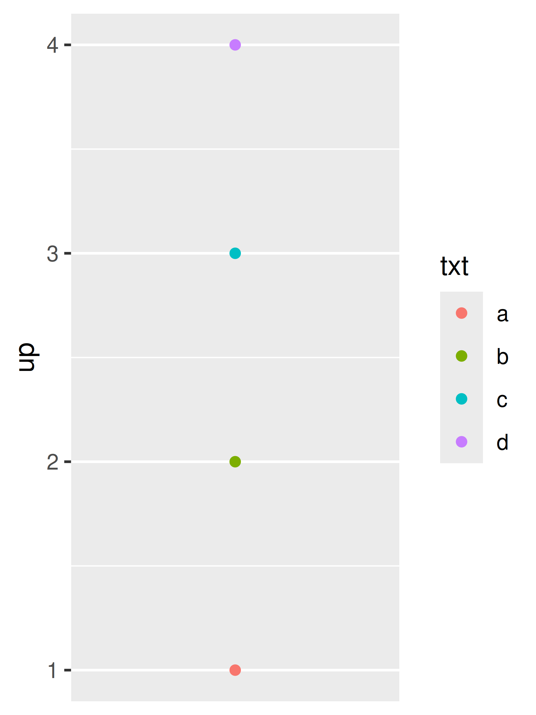

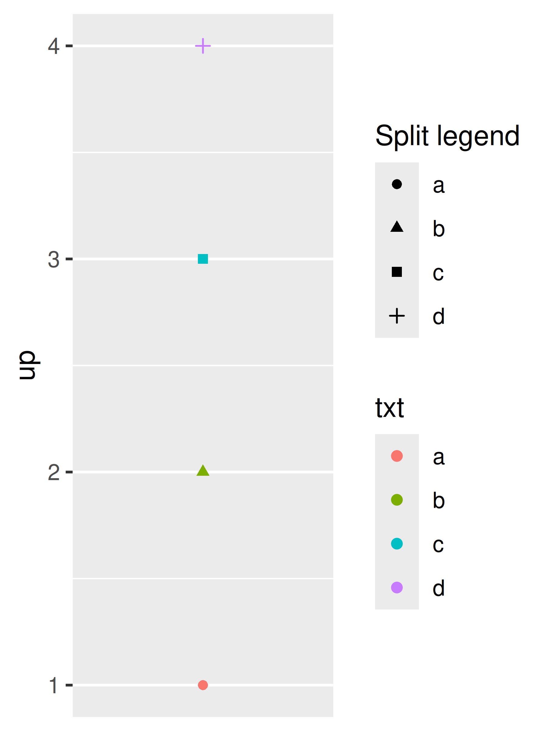
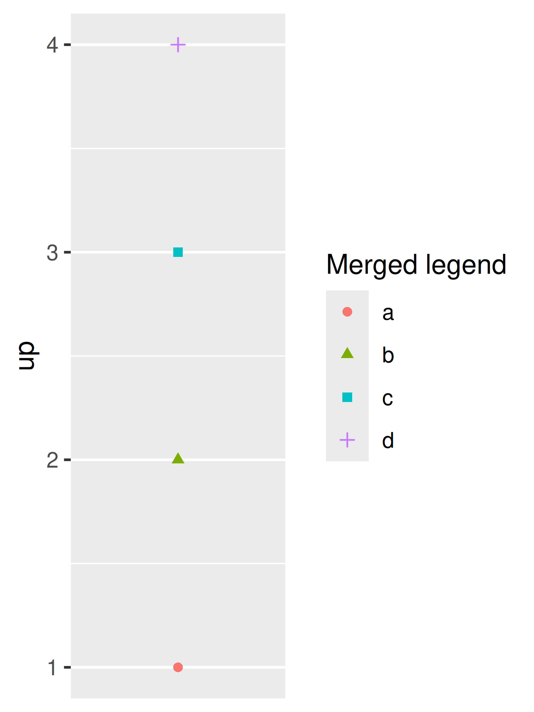
In order for legends to be merged, they must have the same name. So if you change the name of one of the scales, you’ll need to change it for all of them. One way to do this is by using labs() helper function:

base <- ggplot(toy, aes(const, up)) + 
  geom_point(aes(shape = txt, colour = txt)) + 
  scale_x_continuous(NULL, breaks = NULL)

base
base + labs(shape = "Split legend")
base + labs(shape = "Merged legend", colour = "Merged legend")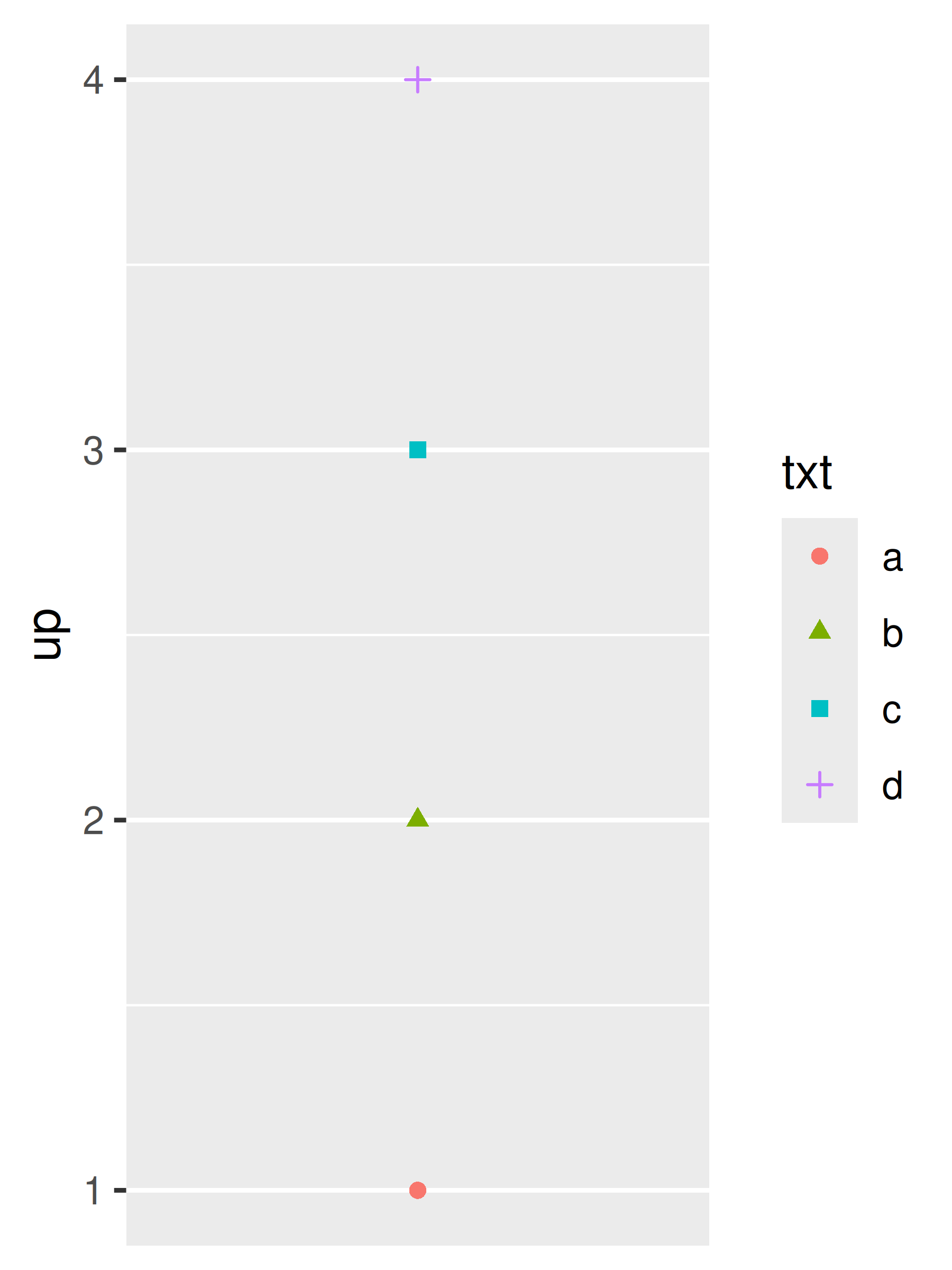

14.7.2 Splitting legends

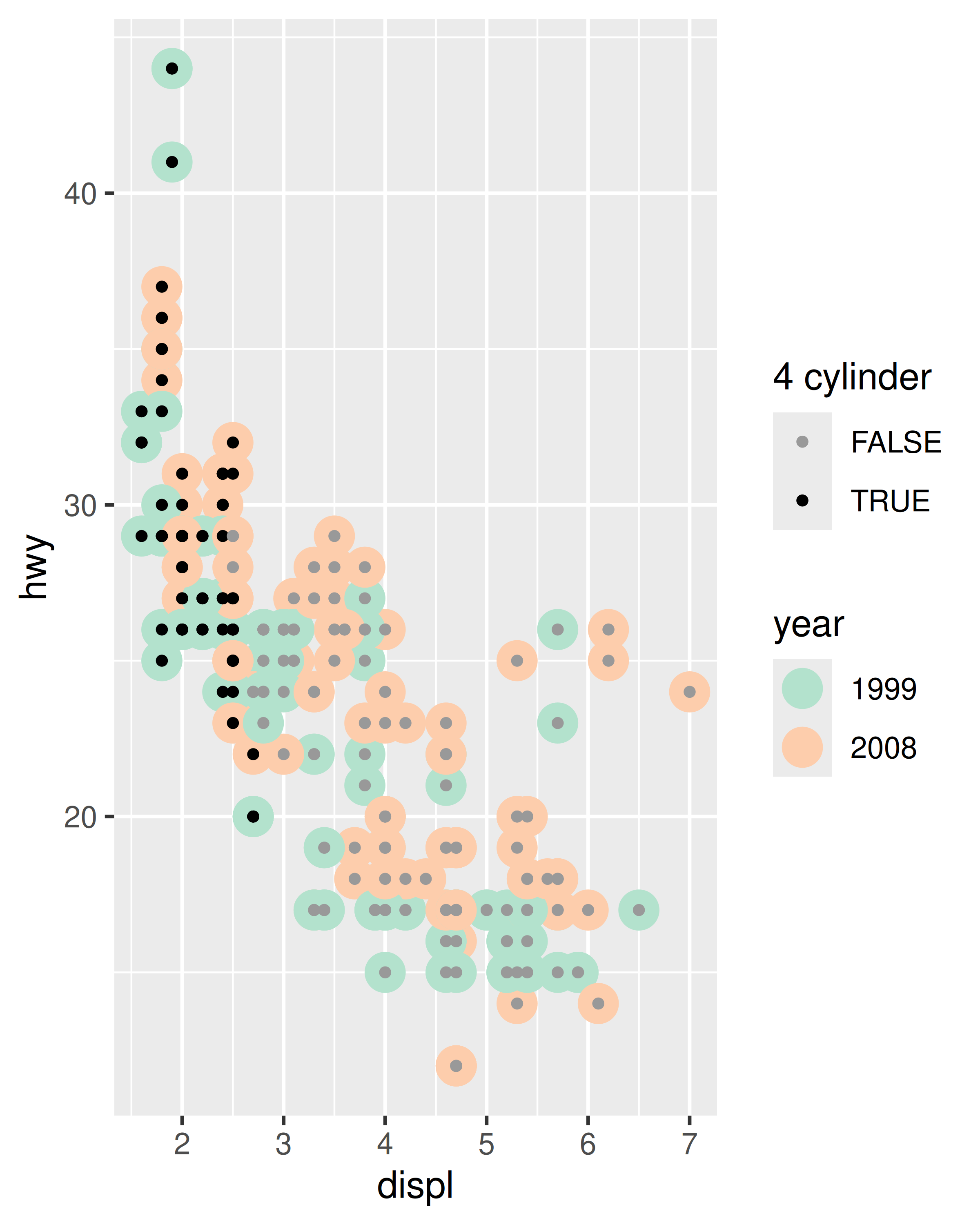
Splitting a legend is a much less common data visualisation task. In general it is not advisable to map one aesthetic (e.g. colour) to multiple variables, and so by default ggplot2 does not allow you to “split” the colour aesthetic into multiple scales with separate legends. Nevertheless, there are exceptions to this general rule, and it is possible to override this behaviour using the ggnewscale package (Campitelli 2020). The ggnewscale::new_scale_colour() command acts as an instruction to ggplot2 to initialise a new colour scale: scale and guide commands that appear above the new_scale_colour() command will be applied to the first colour scale, and commands that appear below are applied to the second colour scale.

To illustrate this the plot on the left uses geom_point() to display a large marker for each vehicle make in the mpg data, with a single colour scale that maps to the year. On the right, a second geom_point() layer is overlaid on the plot using small markers: this layer is associated with a different colour scale, used to indicate whether the vehicle has a 4-cylinder engine.

base <- ggplot(mpg, aes(displ, hwy)) + 
  geom_point(aes(colour = factor(year)), size = 5) + 
  scale_colour_brewer("year", type = "qual", palette = 5) 

base
base + 
  ggnewscale::new_scale_colour() + 
  geom_point(aes(colour = cyl == 4), size = 1, fill = NA) + 
  scale_colour_manual("4 cylinder", values = c("grey60", "black"))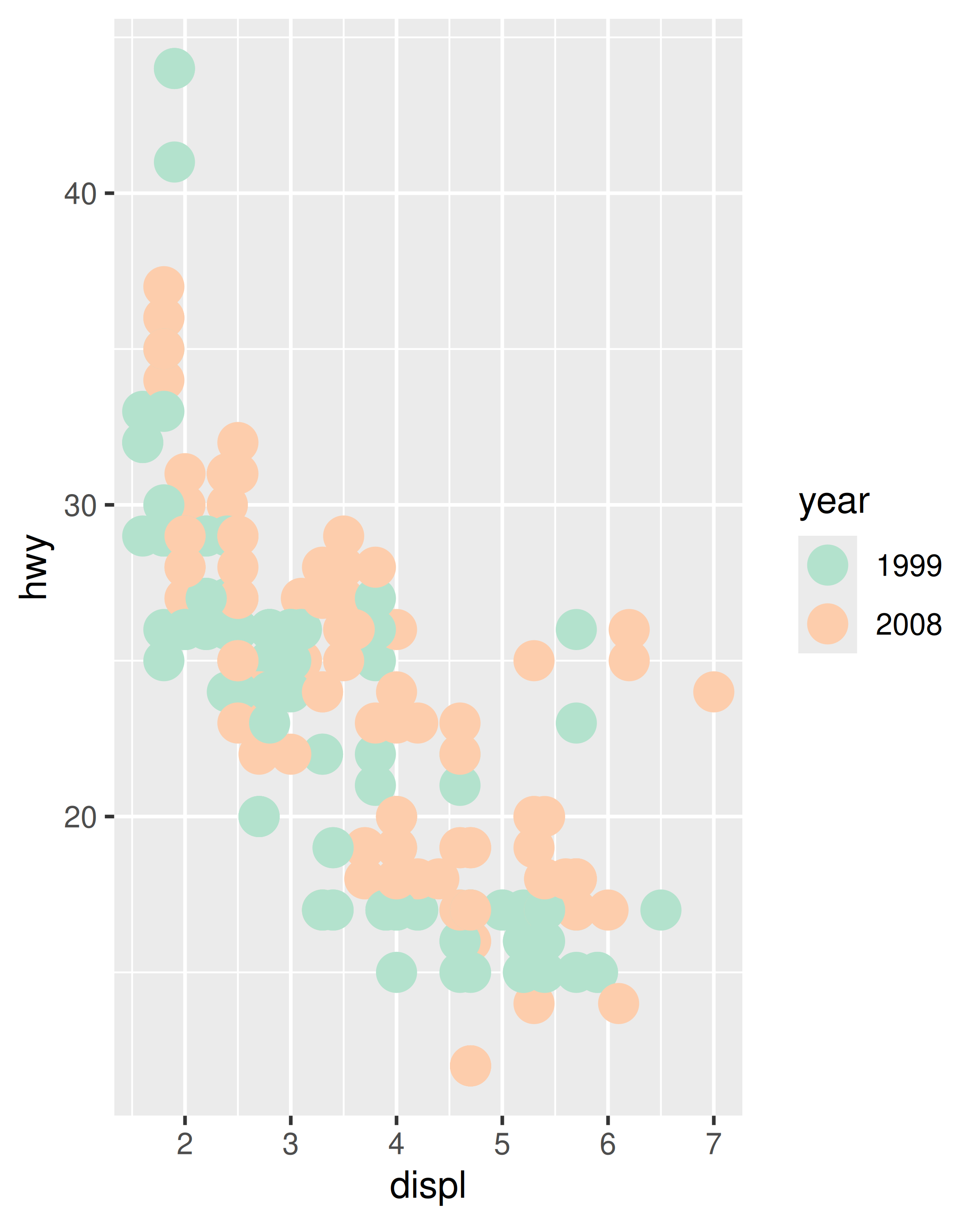

Additional details, including functions that apply to other scale types, are available on the package website, https://github.com/eliocamp/ggnewscale.

14.8 Legend key glyphs

In most cases the default glyphs shown in the legend key will be appropriate to the layer and the aesthetic. Line plots of different colours will show up as lines of different colours in the legend, boxplots will appear as small boxplots in the legend, and so on. Should you need to override this behaviour, the key_glyph argument can be used to associate a particular layer with a different kind of glyph. For example:

base <- ggplot(economics, aes(date, psavert, color = "savings"))

base + geom_line()
base + geom_line(key_glyph = "timeseries")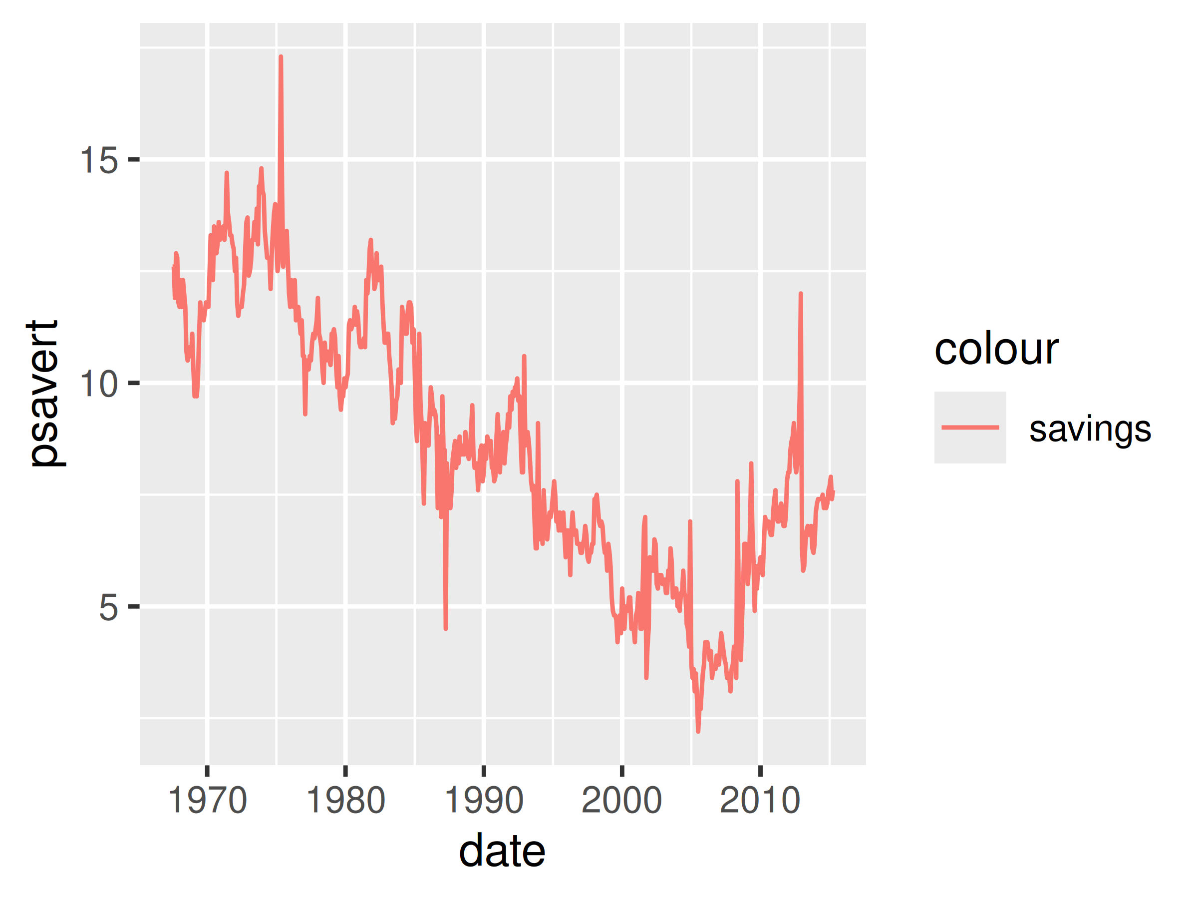

More precisely, each geom is associated with a function such as draw_key_boxplot() or draw_key_path() which is responsible for drawing the key when the legend is created. You can pass the desired key drawing function directly: for example, base + geom_line(key_glyph = draw_key_timeseries) would also produce the plot shown above right.

Campitelli, Elio. 2020. Ggnewscale: Multiple Fill and Colour Scales in ’Ggplot2’. https://CRAN.R-project.org/package=ggnewscale.