11 Colour scales and legends
You are reading the work-in-progress third edition of the ggplot2 book. This chapter should be readable but is currently undergoing final polishing.
After position, the most commonly used aesthetics are those based on colour, and there are many ways to map values to colours in ggplot2. Because colour is complex, the chapter starts with a discussion of colour theory (Section 11.1) with special reference to colour blindness (Section 11.1.1). Mirroring the structure in the previous chapters, the next three sections are dedicated to continuous colour scales (Section 11.2), discrete colour scales (Section 11.3), and binned colour scales (Section 11.4). The chapter concludes by discussing date/time colour scales (Section 11.5), transparency scales (Section 11.6), and the mechanics of legend positioning (Section 11.7).
11.1 A little colour theory
Before we look at the details, it’s useful to learn a little bit of colour theory. Colour theory is complex because the underlying biology of the eye and brain is complex, and this introduction will only touch on some of the more important issues. An excellent and more detailed exposition is available online at http://tinyurl.com/clrdtls.
At the physical level, colour is produced by a mixture of wavelengths of light. To characterise a colour completely, we need to know the complete mixture of wavelengths. Fortunately for us the human eye only has three different colour receptors, and so we can summarise the perception of any colour with just three numbers. You may be familiar with the RGB encoding of colour space, which defines a colour by the intensities of red, green and blue light needed to produce it. One problem with this space is that it is not perceptually uniform: the two colours that are one unit apart may look similar or very different depending on where they are in the colour space. This makes it difficult to create a mapping from a continuous variable to a set of colours. There have been many attempts to come up with colours spaces that are more perceptually uniform. We’ll use a modern attempt called the HCL colour space, which has three components of hue, chroma and luminance:
- Hue ranges from 0 to 360 (an angle) and gives the “colour” of the colour (blue, red, orange, etc).
- Chroma is the “purity” of a colour, ranging from 0 (grey) to a maximum that varies with luminance.
- Luminance is the lightness of the colour, ranging from 0 (black) to 1 (white).
The three dimensions have different properties. Hues are arranged around a colour wheel and are not perceived as ordered: e.g. green does not seem “larger” than red, and blue does not seem to be “in between” green or red. In contrast, both chroma and luminance are perceived as ordered: pink is perceived as lying between red and white, and grey is seen to fall between black and white.
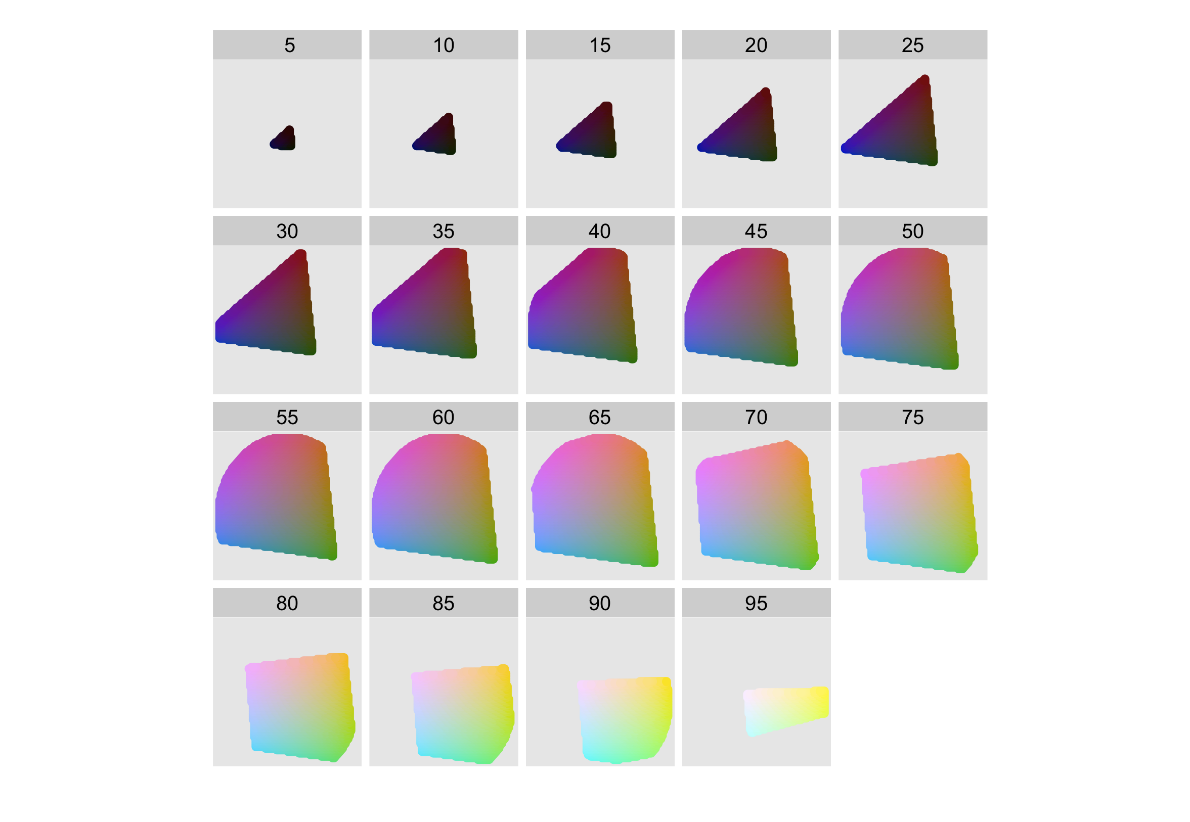
The combination of these three components does not produce a simple geometric shape. The figure below attempts to show the 3d shape of the space. Each slice is a constant luminance (brightness) with hue mapped to angle and chroma to radius. You can see the centre of each slice is grey and the colours get more intense as they get closer to the edge.
11.1.1 Colour blindness
An additional complication is that a sizeable minority of people do not possess the usual complement of colour receptors and so can distinguish fewer colours than others. Because of this, it is important to consider how a colour palette will look to people with common forms of colour blindness. A simple heuristic is to avoid red-green contrasts, and to check your plots with systems that simulate colour blindness. In addition to the many online tools that can assist with this (e.g., https://www.vischeck.com/), there are several R packages provide tools you may find helpful. The dichromat package (Lumley 2007) provides tools for simulating colour blindness, and a set of colour schemes known to work well for colour-blind people. Another useful tool is the colorBlindness package (Ou 2021) which provides a displayAllColors() function that helps you approximate the appearance of a given set of colours under different forms of colour blindness. As an illustration, it quickly reveals that colours provided by the rainbow() palette are not appropriate if you are trying to create plots that are readable by colour blind people, nor do they reproduce well in greyscale:
colorBlindness::displayAllColors(rainbow(6))
By way of contrast, colours provided by viridis::viridis() are discriminable under the most common forms of colour blindness, and reproduce well in greyscale:
colorBlindness::displayAllColors(viridis::viridis(6))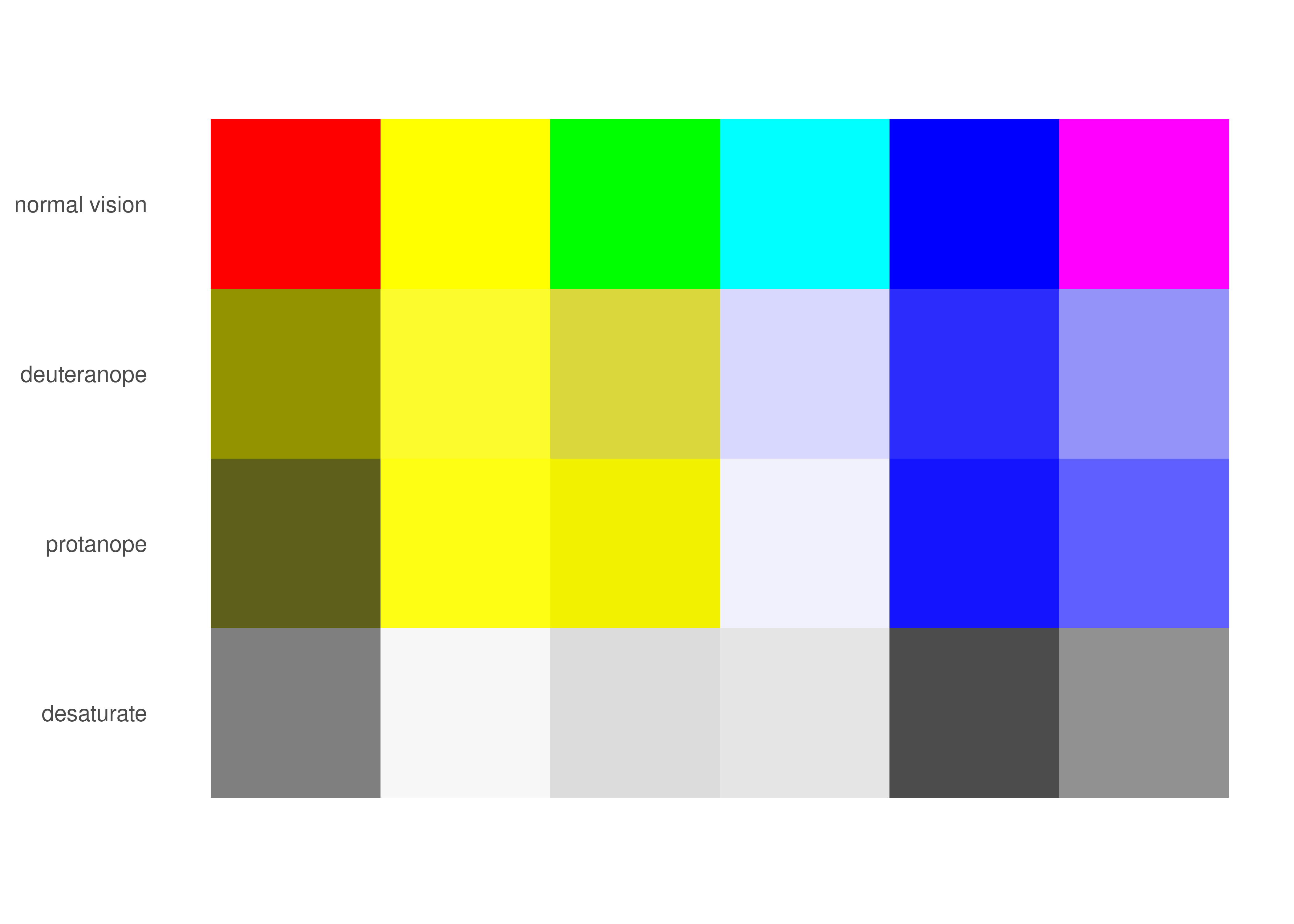
In addition to the viridis package there are other R packages that provide palettes that are explicitly colour blind safe, and you’ll see these in use throughout the chapter. Finally, you can also help people with colour blindness in the same way that you can help people with black-and-white printers: by providing redundant mappings to other aesthetics like size, line type or shape.
11.2 Continuous colour scales
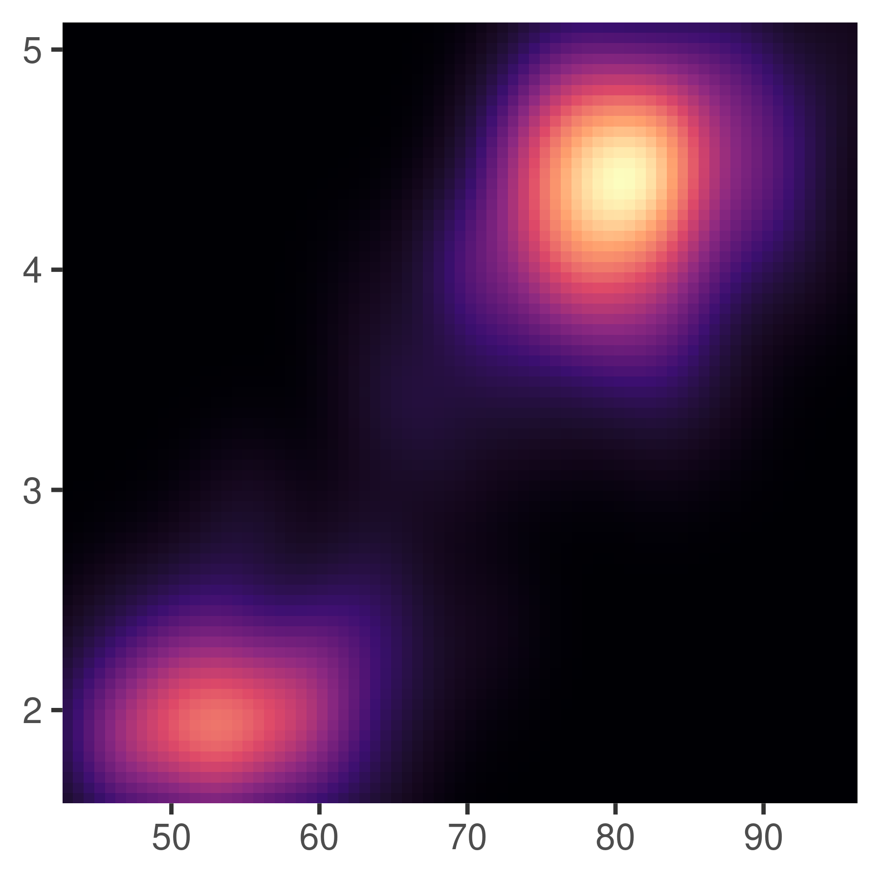
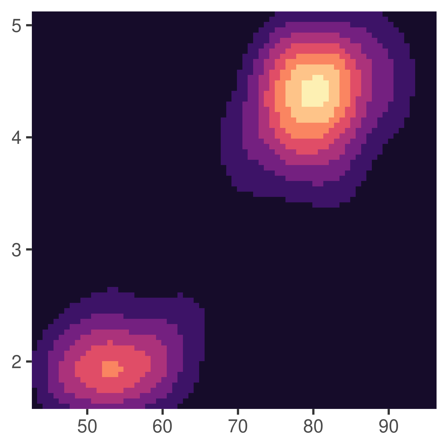
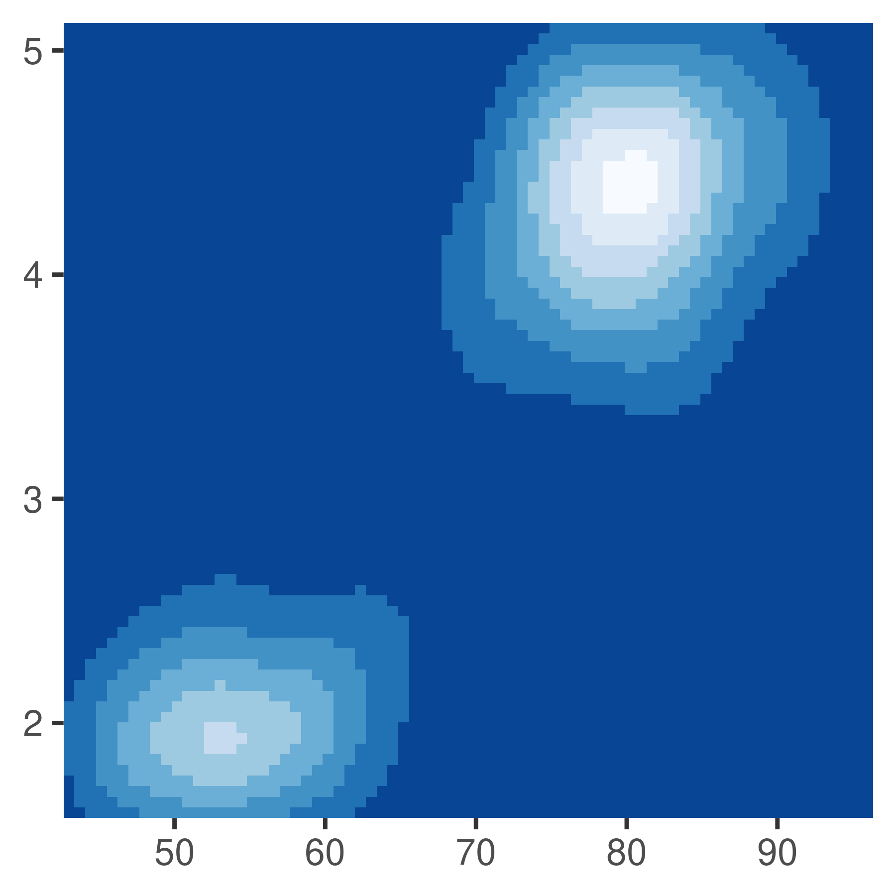
Colour gradients are often used to show the height of a 2d surface. The plots in this section use the surface of a 2d density estimate of the faithful dataset (Azzalini and Bowman 1990), which records the waiting time between eruptions and during each eruption for the Old Faithful geyser in Yellowstone Park. We hide the legends and set expand to 0, to focus on the appearance of the data. Remember: although we use the erupt plot to illustrate concepts using with a fill aesthetic, the same ideas apply to colour scales. Any time we refer to scale_fill_*() in this section there is a corresponding scale_colour_*() for the colour aesthetic (or scale_color_*() if you prefer US spelling).
11.2.1 Particular palettes
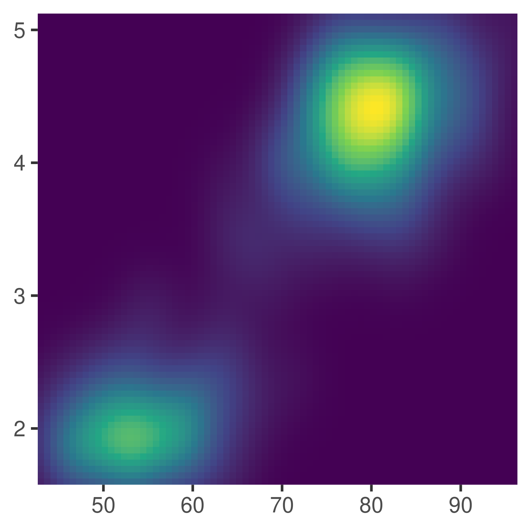
There are multiple ways to specify continuous colour scales. Later we’ll talk about general purpose tools that you can use to construct your own palette, but this is often unnecessary as there are many “hand picked” palettes available. For example, ggplot2 supplies two scale functions that bundle pre-specified palettes, scale_fill_viridis_c() and scale_fill_distiller(). The viridis scales (Garnier 2018) are designed to be perceptually uniform in both colour and when reduced to black and white, and to be perceptible to people with various forms of colour blindness.
erupt
erupt + scale_fill_viridis_c()
erupt + scale_fill_viridis_c(option = "magma")


For most use cases, the viridis scales will work better than other continuous scales built into ggplot2, but there are other options that are useful in some situations. A second group of continuous colour scales built in to ggplot2 are derived from the ColorBrewer scales: scale_fill_brewer() provides these colours as discrete palettes, while scale_fill_distiller() and scale_fill_fermenter() are the continuous and binned analogs. We discuss these scales in Section 11.3, but for illustrative purposes include some examples here:
erupt + scale_fill_distiller()
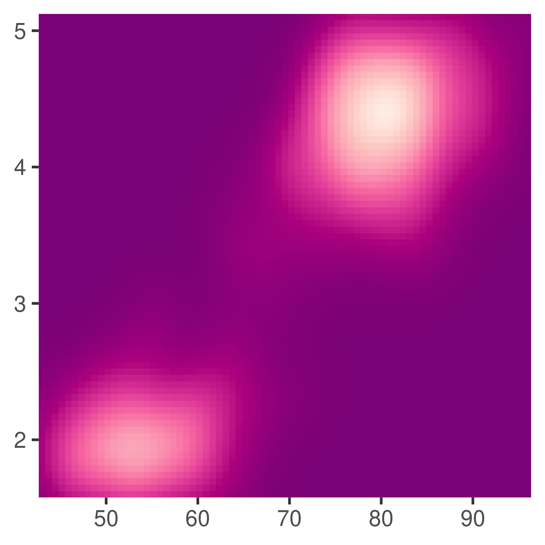
erupt + scale_fill_distiller(palette = "RdPu")
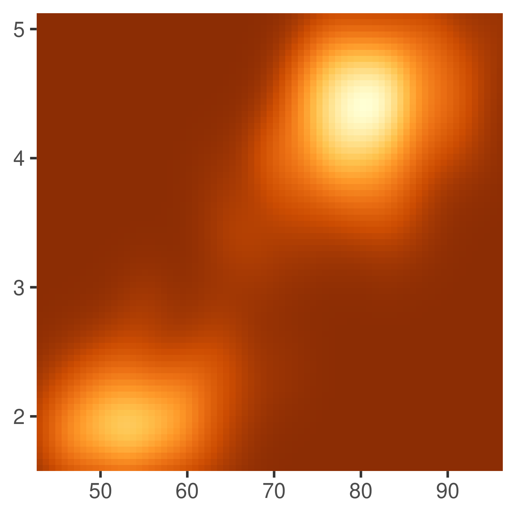
erupt + scale_fill_distiller(palette = "YlOrBr")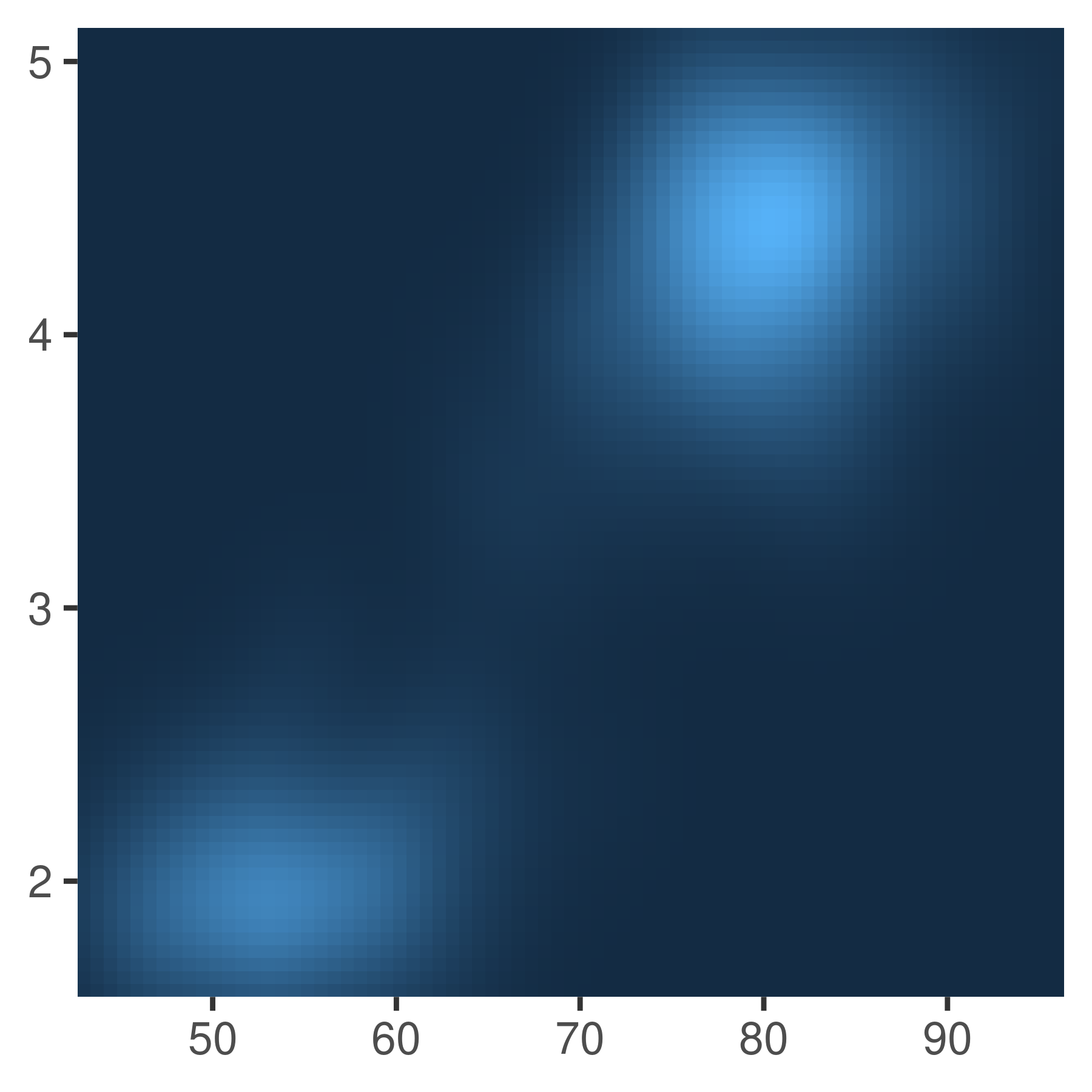
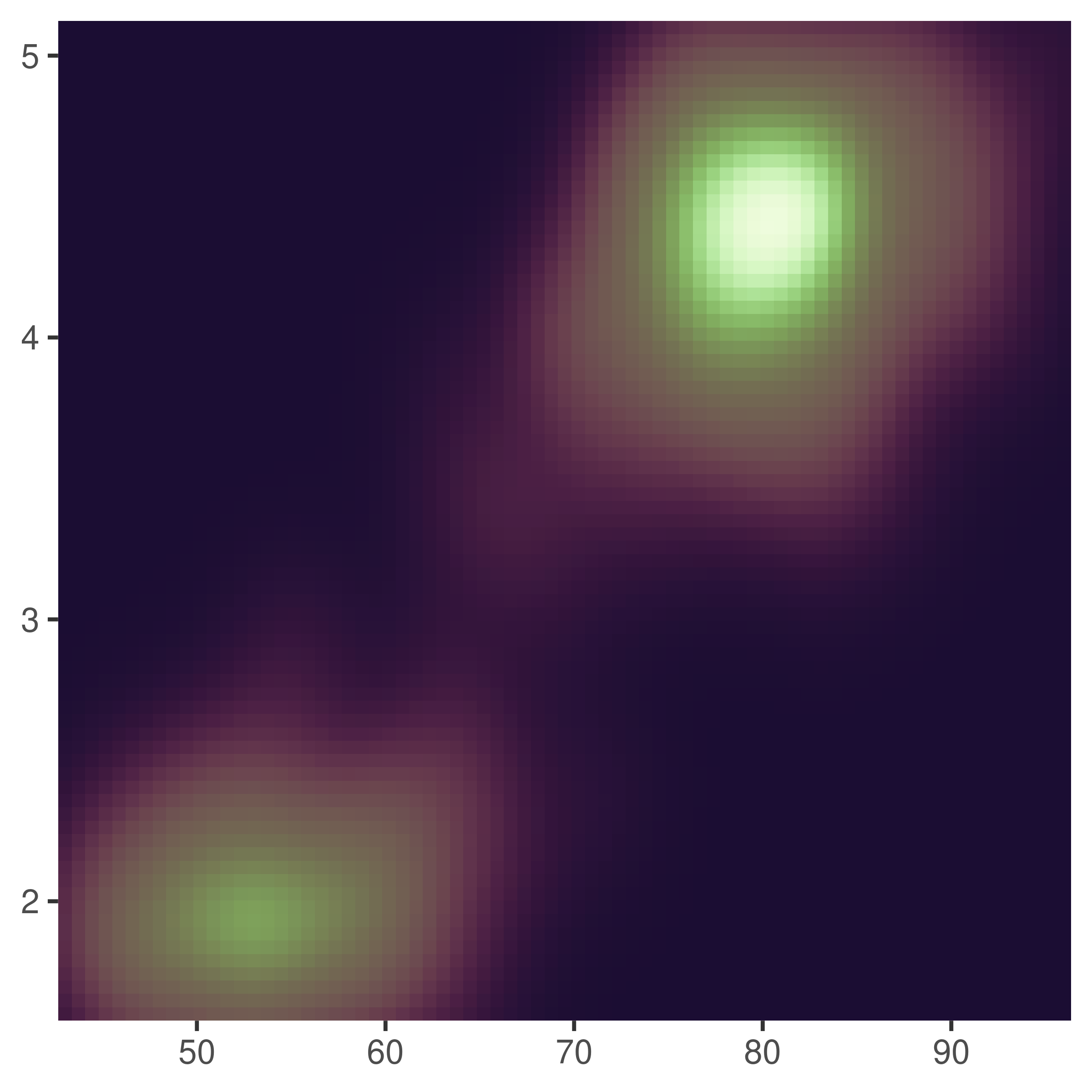
There are many other packages that provide useful colour palettes. For example, scico (Pedersen and Crameri 2020) provides more palettes that are perceptually uniform and suitable for scientific visualisation:
erupt + scico::scale_fill_scico(palette = "bilbao") # the default
erupt + scico::scale_fill_scico(palette = "vik")
erupt + scico::scale_fill_scico(palette = "lajolla")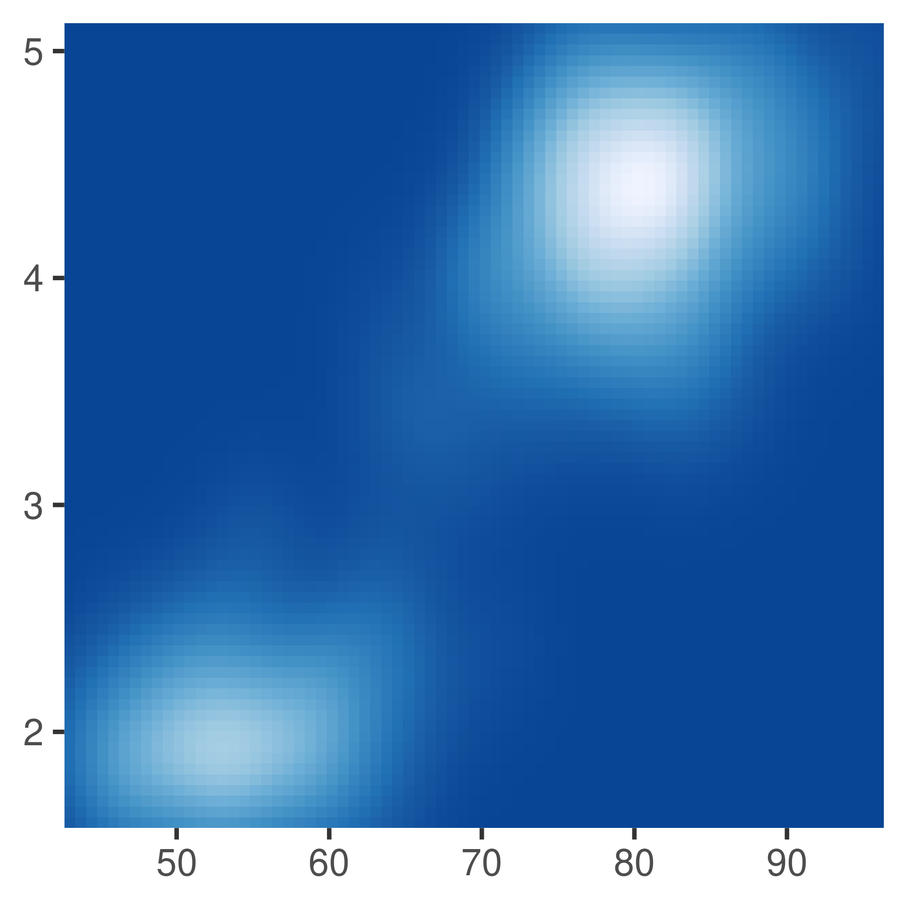
However, as there are a great many palette packages in R, a particularly useful package is paletteer (Hvitfeldt 2020), which aims to provide a common interface:
erupt + paletteer::scale_fill_paletteer_c("viridis::plasma")
erupt + paletteer::scale_fill_paletteer_c("scico::tokyo")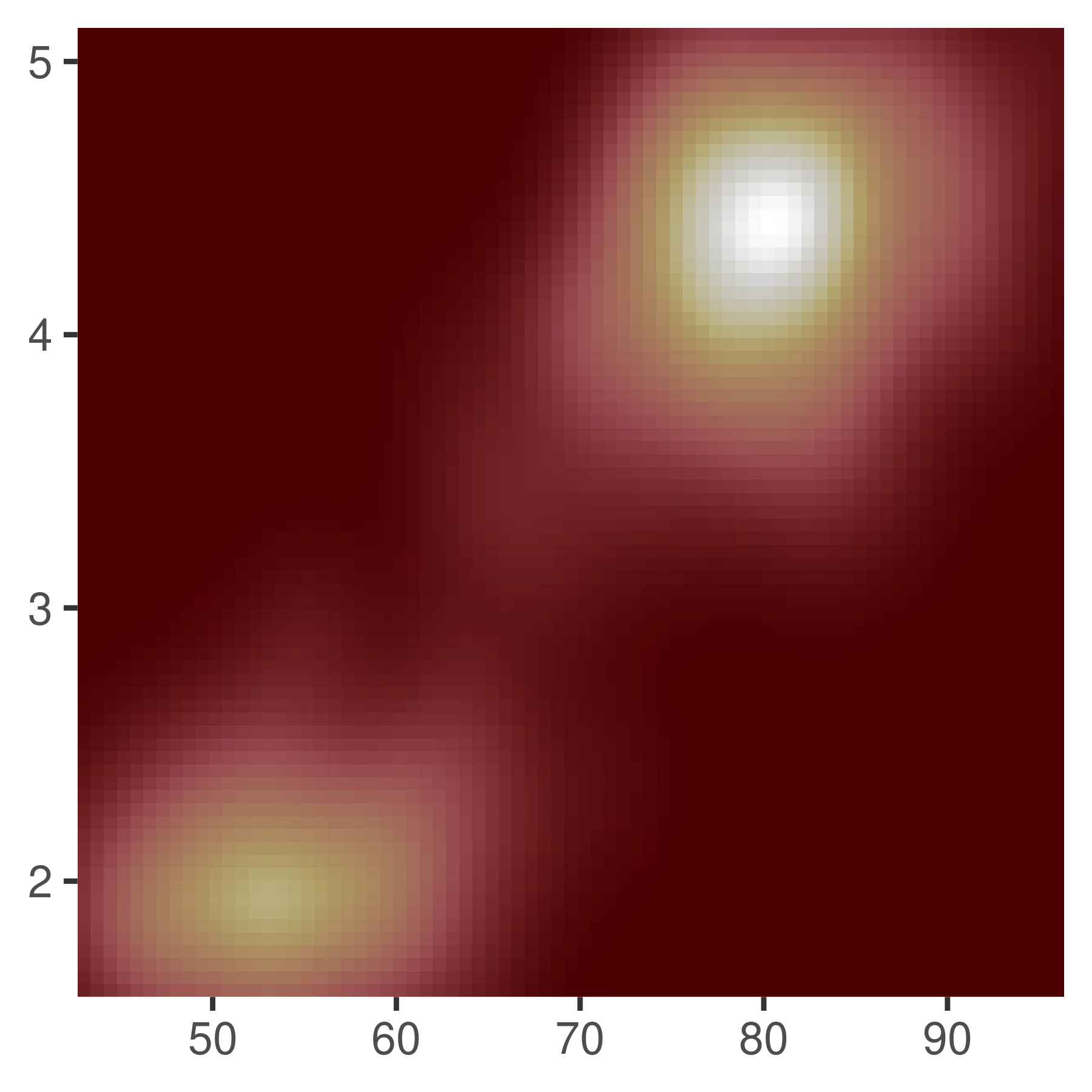
11.2.2 Robust recipes
The default scale for continuous fill scales is scale_fill_continuous() which in turn defaults to scale_fill_gradient(). As a consequence, these three commands produce the same plot using a gradient scale:
erupt
erupt + scale_fill_continuous()
erupt + scale_fill_gradient()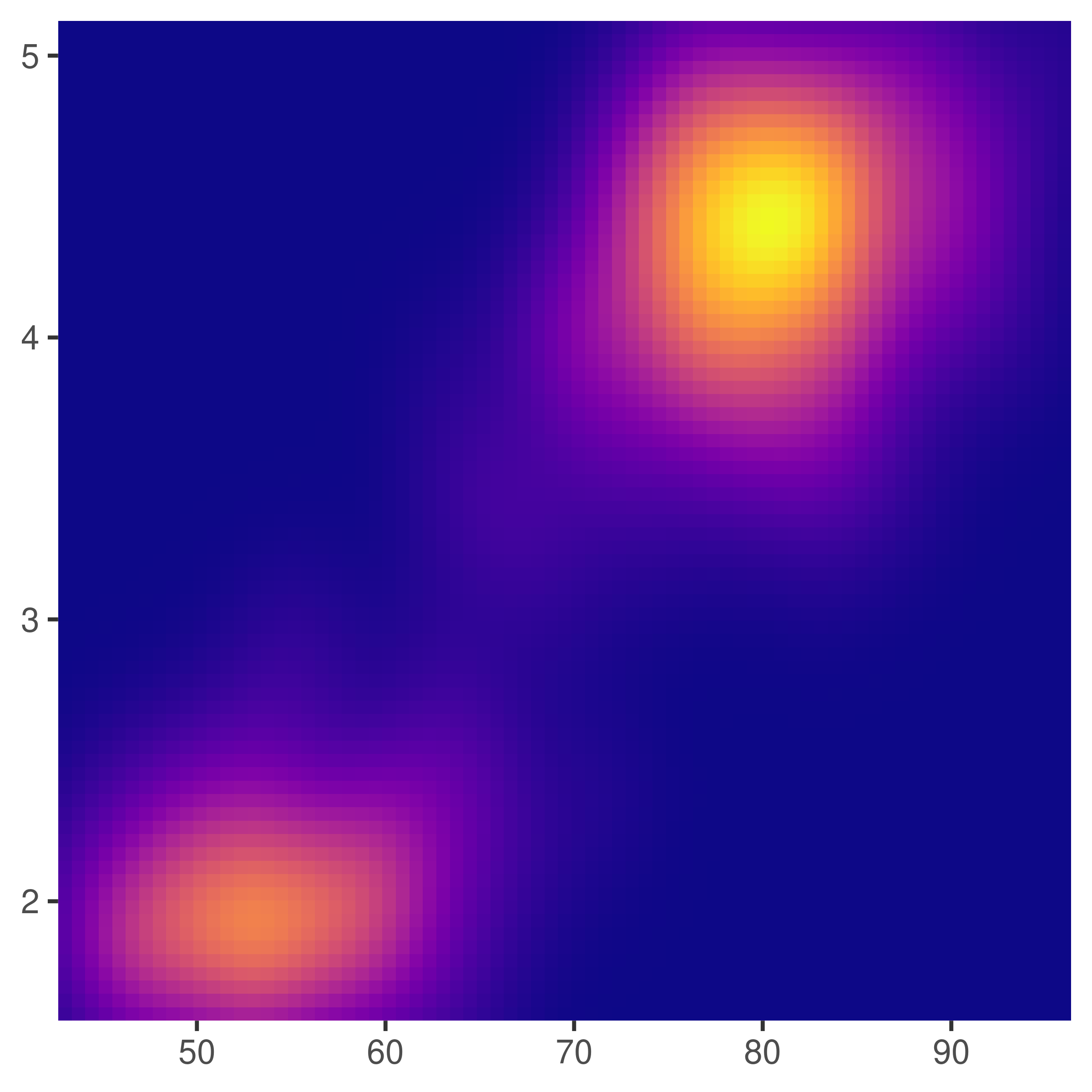

Gradient scales provide a robust method for creating any colour scheme you like. All you need to do is specify two or more reference colours, and ggplot2 will interpolate linearly between them. There are three functions that you can use for this purpose:
-
scale_fill_gradient()produces a two-colour gradient -
scale_fill_gradient2()produces a three-colour gradient with specified midpoint -
scale_fill_gradientn()produces an n-colour gradient
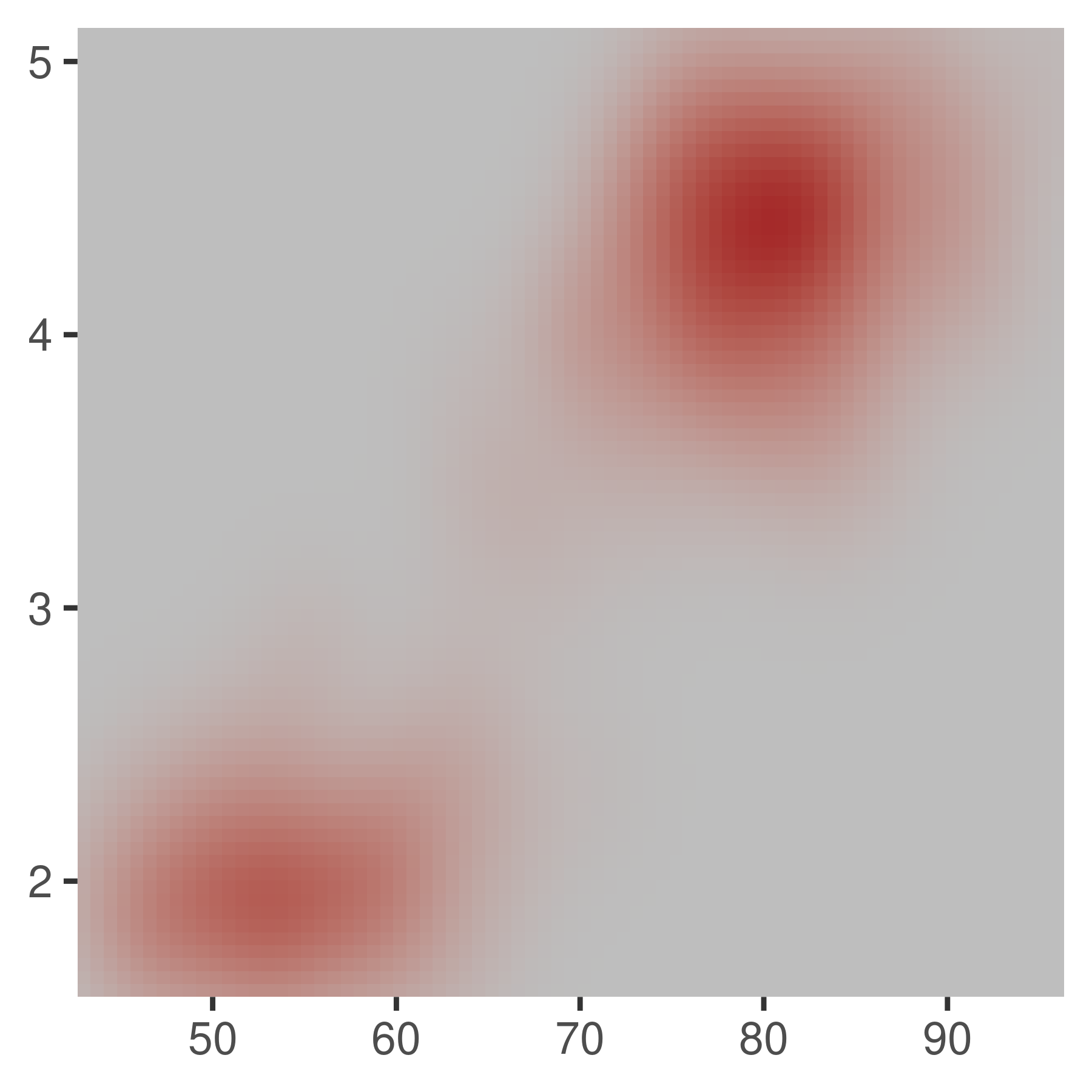
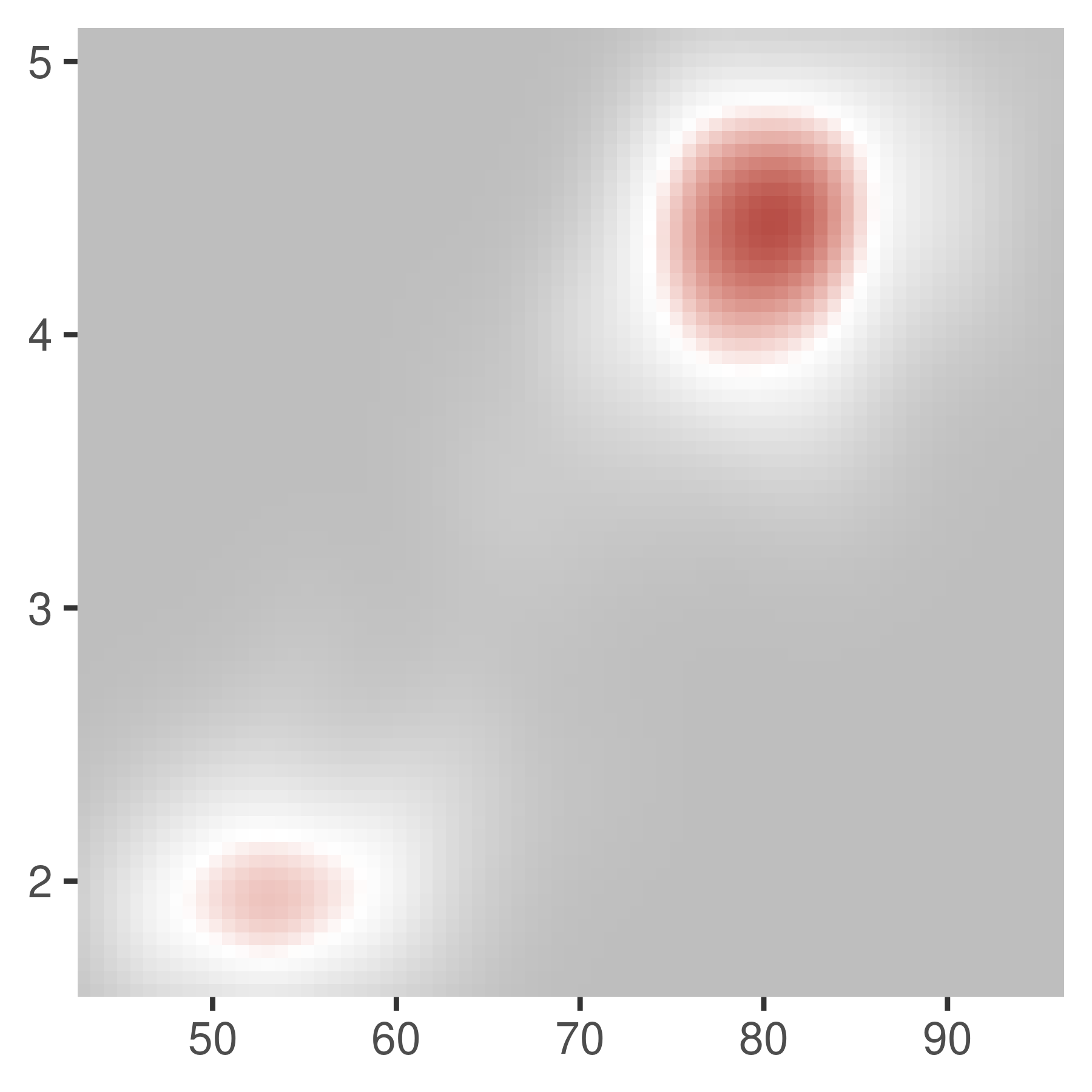
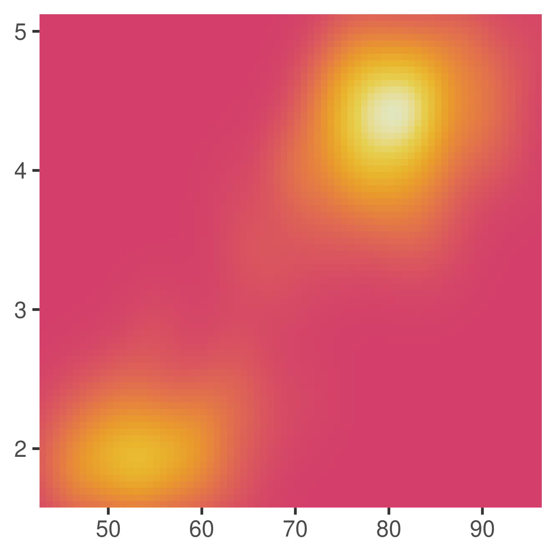
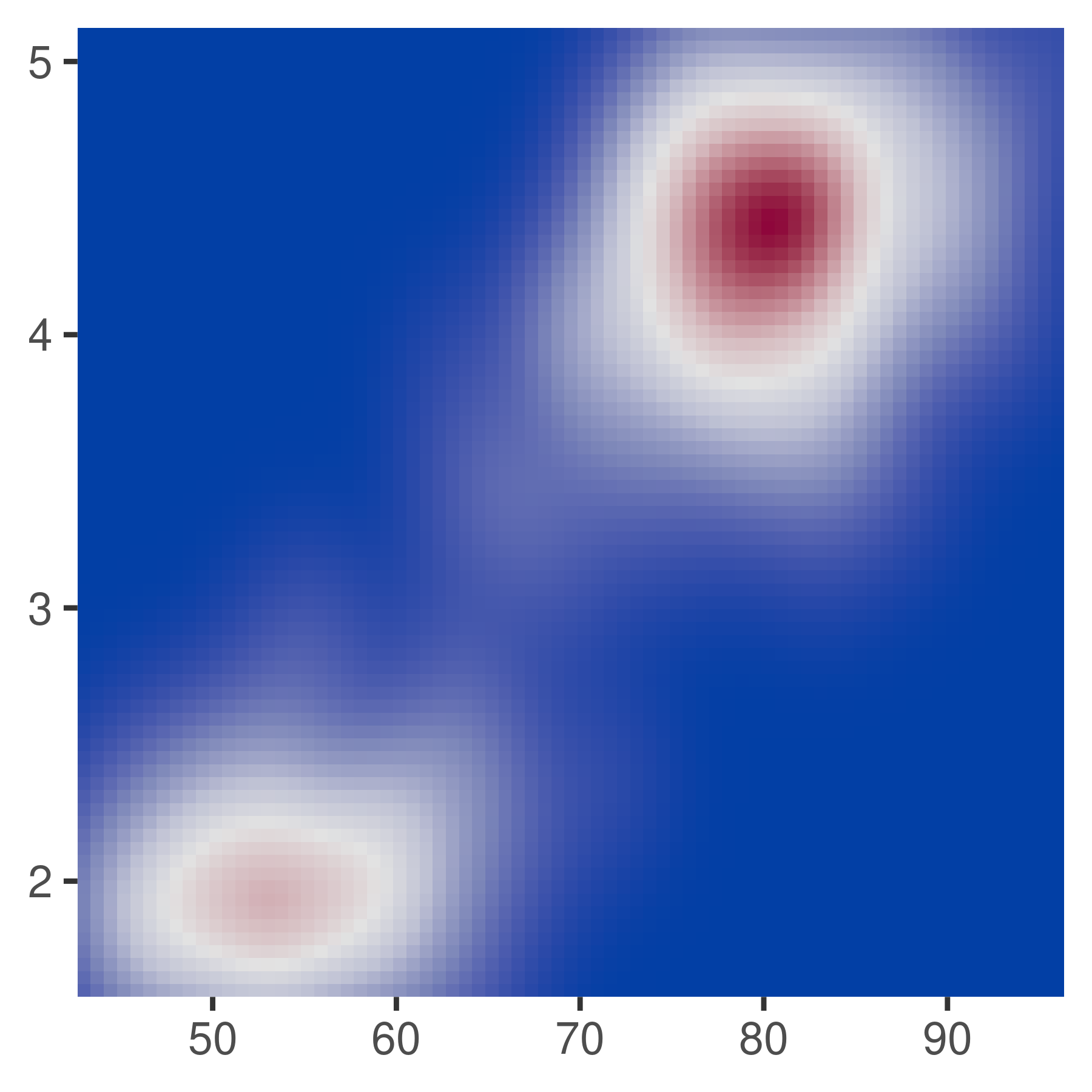
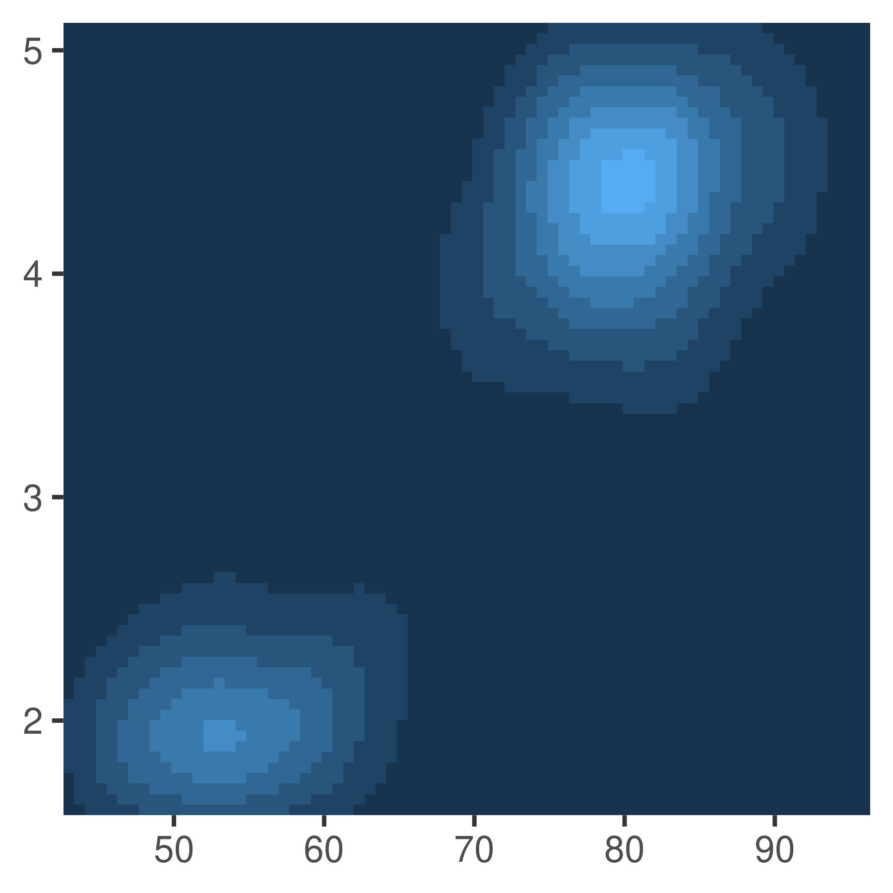
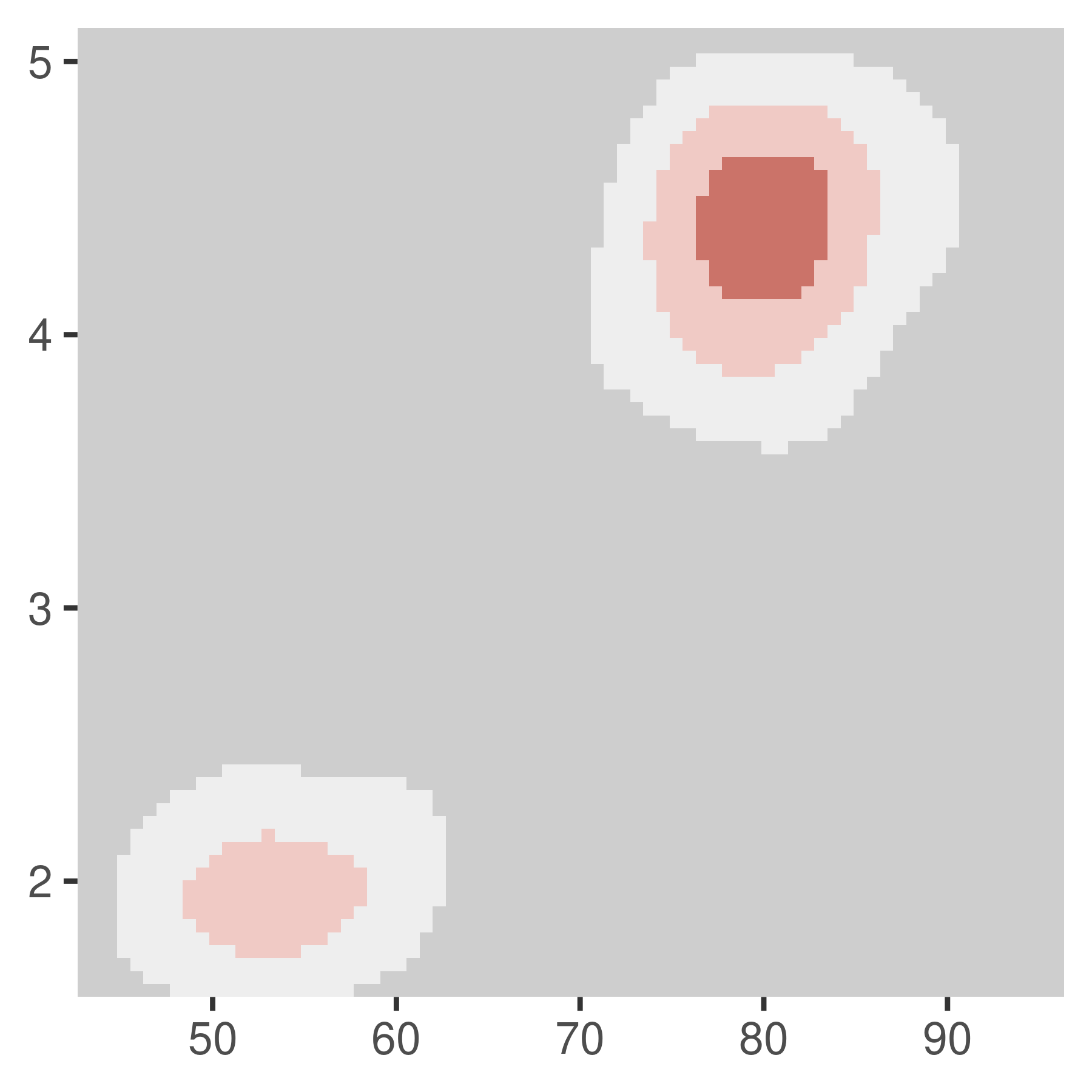
The use of gradient scales is illustrated below. The first plot uses a scale that linearly interpolates from grey (hex code: "#bebebe") at the low end of the scale limits to brown ("#a52a2a") at the high end. The second plot has the same endpoints but uses scale_fill_gradient2() to interpolate first from grey to white (#ffffff) and then from white to brown. Note that the mid argument specifies the colour to be shown at the intermediate point, and midpoint is the value in the data at which this colour is used (the default is midpoint = 0). The third method is to use scale_fill_gradientn() which takes a vector of reference colours as its argument, and constructs a scale that linearly interpolates between the specified values. By default, the colours are presumed to be equally spaced along the scale, but if you prefer you can specify a vector of values that correspond to each of the reference colours.
erupt + scale_fill_gradient(low = "grey", high = "brown")
erupt +
  scale_fill_gradient2(
    low = "grey",
    mid = "white",
    high = "brown",
    midpoint = .02
  )
erupt + scale_fill_gradientn(colours = terrain.colors(7))


Creating good colour palettes requires some care. Generally, for a two-point gradient scale you want to convey the perceptual impression that the values are sequentially ordered, so you want to keep hue constant, and vary chroma and luminance. The Munsell colour system is useful for this as it provides an easy way of specifying colours based on their hue, chroma and luminance. The munsell package (Wickham 2018) provides easy access to the Munsell colours, which can then be used to specify a gradient scale:
munsell::hue_slice("5P") +  # Generate a ggplot with hue_slice()
  annotate(                 # Add arrows for annotation
    geom = "segment",
    x = c(7, 7),
    y = c(1, 10),
    xend = c(7, 7),
    yend = c(2, 9),
    arrow = arrow(length = unit(2, "mm"))
  )
#> Warning: Using `size` aesthetic for lines was deprecated in ggplot2 3.4.0.
#> ℹ Please use `linewidth` instead.
#> ℹ The deprecated feature was likely used in the munsell package.
#>   Please report the issue at <https://github.com/cwickham/munsell/issues>.
#> Warning: Removed 31 rows containing missing values or values outside the scale range
#> (`geom_text()`).

# Construct scale
erupt + scale_fill_gradient(
  low = munsell::mnsl("5P 2/12"),
  high = munsell::mnsl("5P 7/12")
)
The labels on the left plot are a little difficult to read at this scale, so we have used annotate() to add arrows highlighting the column used to construct the scale on the right. For more information on the munsell package see https://github.com/cwickham/munsell/.
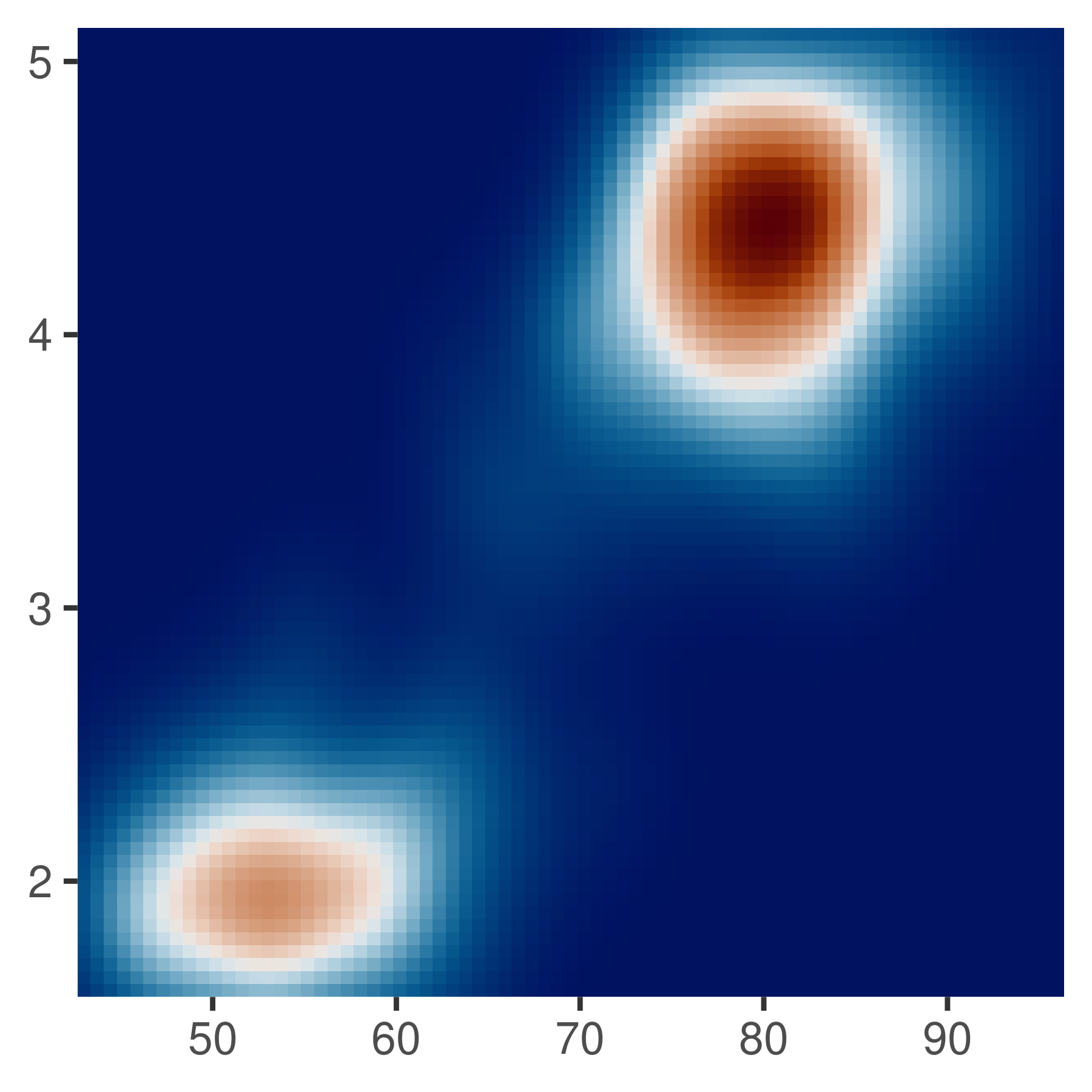
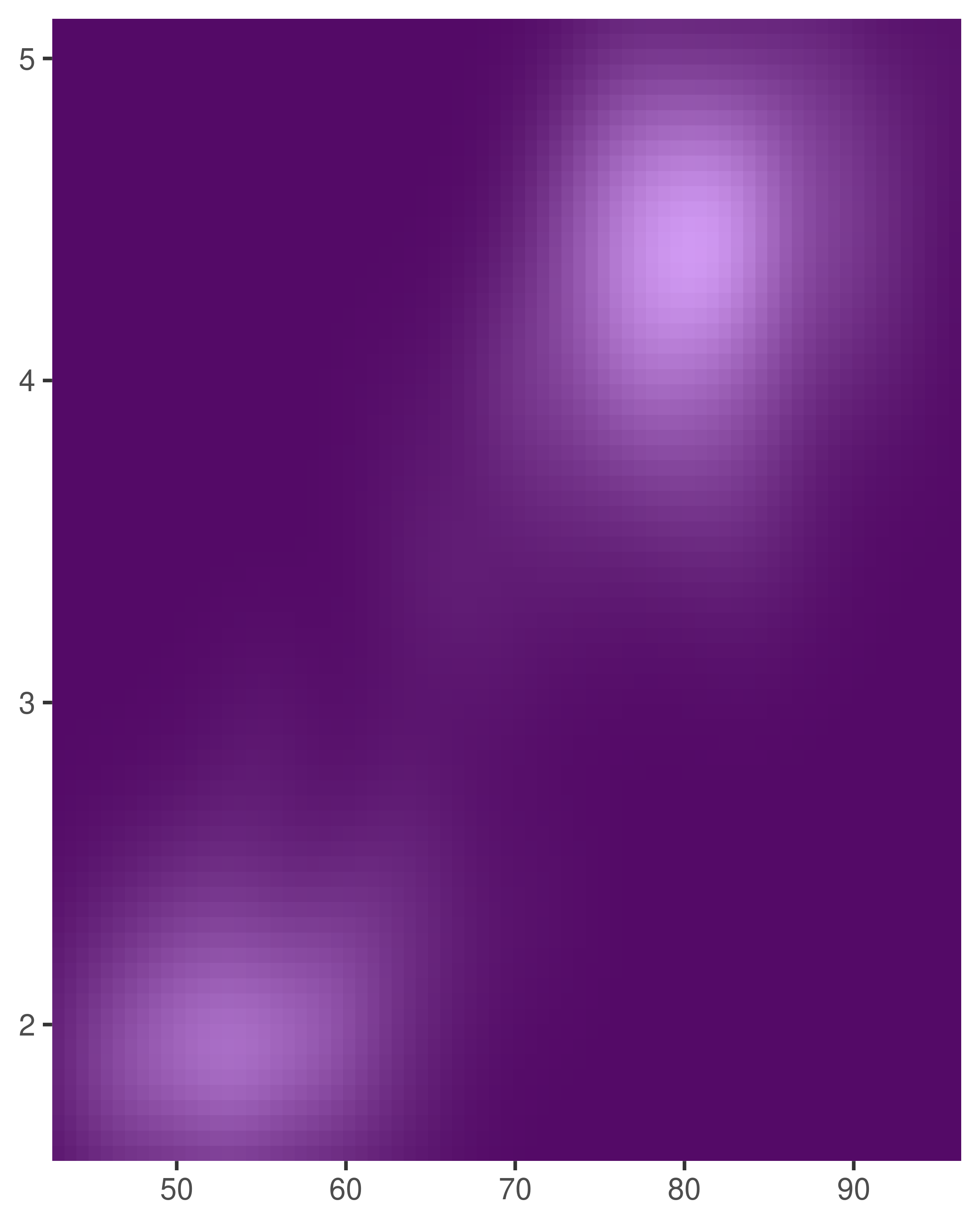
Three-point gradient scales have slightly different design criteria. Typically, the goal in such a scale is to convey the perceptual impression that there is a natural midpoint (often a zero value) from which the other values diverge. The left plot below shows how to create a divergent “yellow/blue” scale, though it is a little artificial in this example.
Finally, if you have colours that are meaningful for your data (e.g., black body colours or standard terrain colours), or you’d like to use a palette produced by another package, you may wish to use an n-point gradient. As an illustration, the middle and right plots below use the colorspace package (Zeileis et al. 2008). For more information on the colorspace package see https://colorspace.r-forge.r-project.org/.
# munsell example
erupt + scale_fill_gradient2(
  low = munsell::mnsl("5B 7/8"),
  high = munsell::mnsl("5Y 7/8"),
  mid = munsell::mnsl("N 7/0"),
  midpoint = .02
)

# colorspace examples
erupt + scale_fill_gradientn(colours = colorspace::heat_hcl(7))
erupt + scale_fill_gradientn(colours = colorspace::diverge_hcl(7))

11.2.3 Missing values
All continuous colour scales have an na.value parameter that controls what colour is used for missing values (including values outside the range of the scale limits). By default it is set to grey, which will stand out when you use a colourful scale. If you use a black and white scale, you might want to set it to something else to make it more obvious. You can set na.value = NA to make missing values invisible, or choose a specific colour if you prefer:
df <- data.frame(x = 1, y = 1:5, z = c(1, 3, 2, NA, 5))
base <- ggplot(df, aes(x, y)) +
  geom_tile(aes(fill = z), linewidth = 5) +
  labs(x = NULL, y = NULL) +
  scale_x_continuous(labels = NULL)

base
base + scale_fill_gradient(na.value = NA)
base + scale_fill_gradient(na.value = "yellow")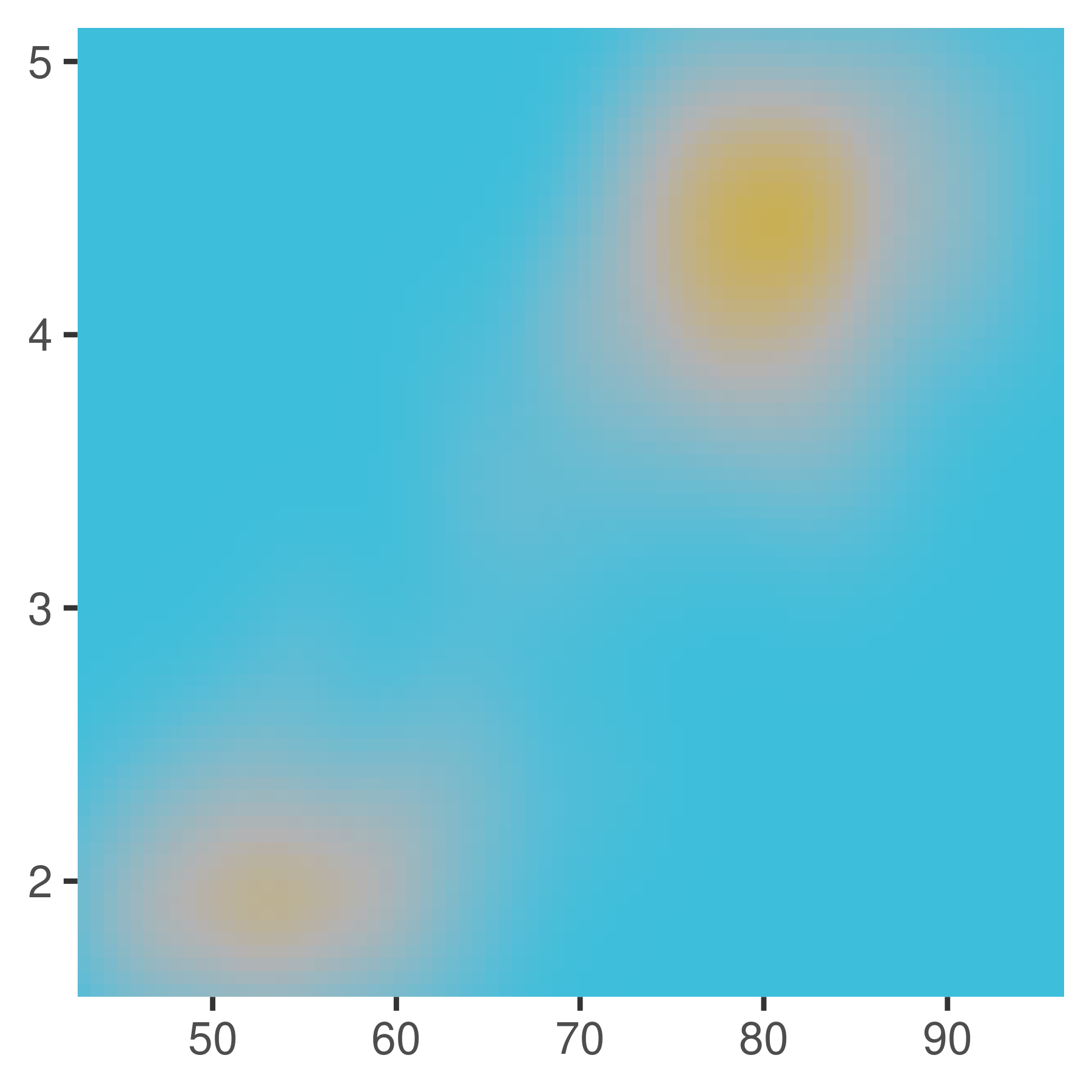
11.2.4 Limits, breaks, and labels
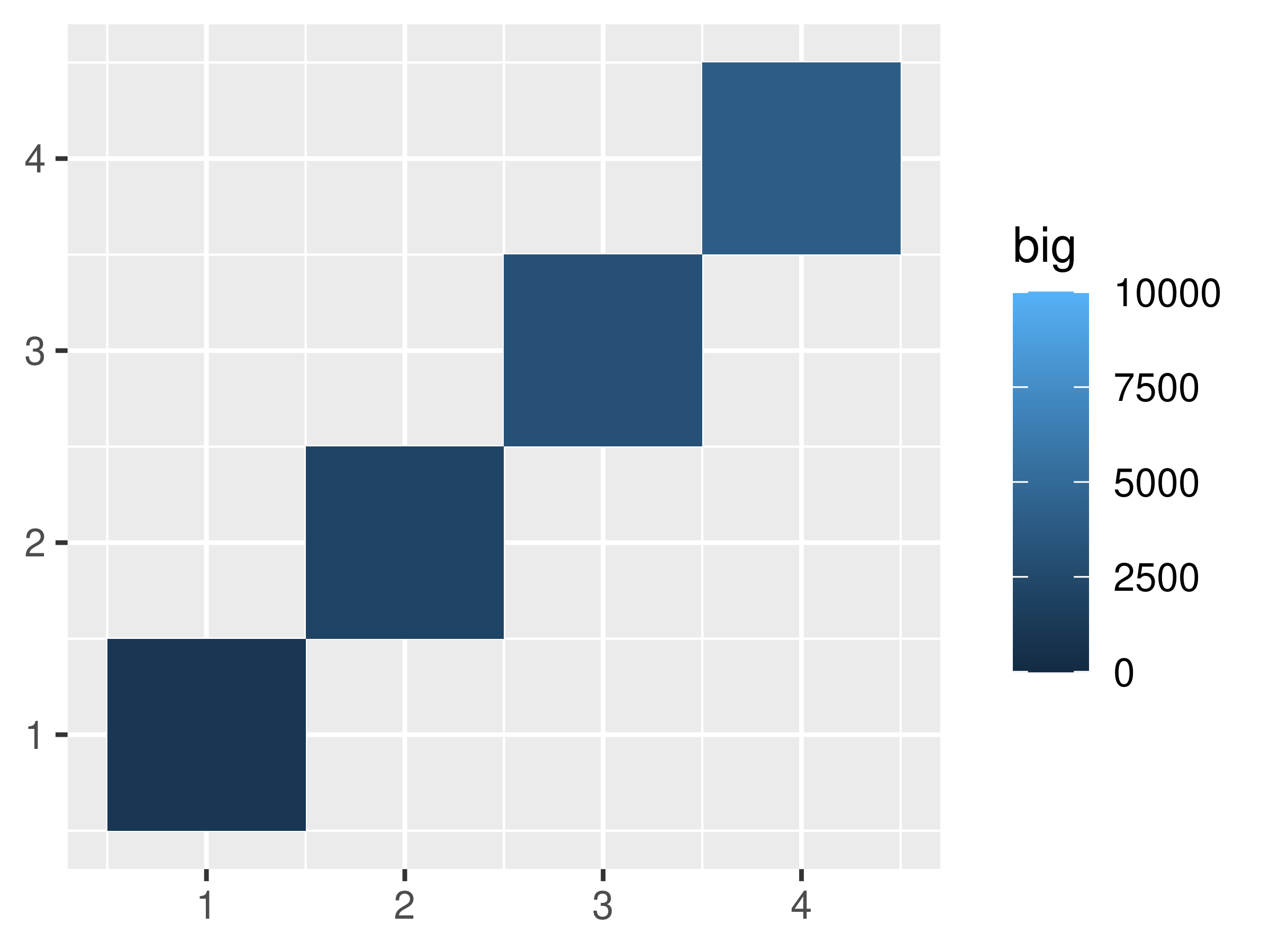
In the previous chapter we discussed how the appearance of axes can be controlled by setting the limits (Section 10.1.1), breaks (Section 10.1.4) and labels (Section 10.1.6) argument to the scale function. The behaviour of colour scales can be controlled in an analogous fashion:
base <- ggplot(toy, aes(up, up, fill = big)) +
  geom_tile() +
  labs(x = NULL, y = NULL)

base
base + scale_fill_continuous(limits = c(0, 10000))

base + scale_fill_continuous(breaks = c(1000, 2000, 4000))
base + scale_fill_continuous(labels = scales::label_dollar())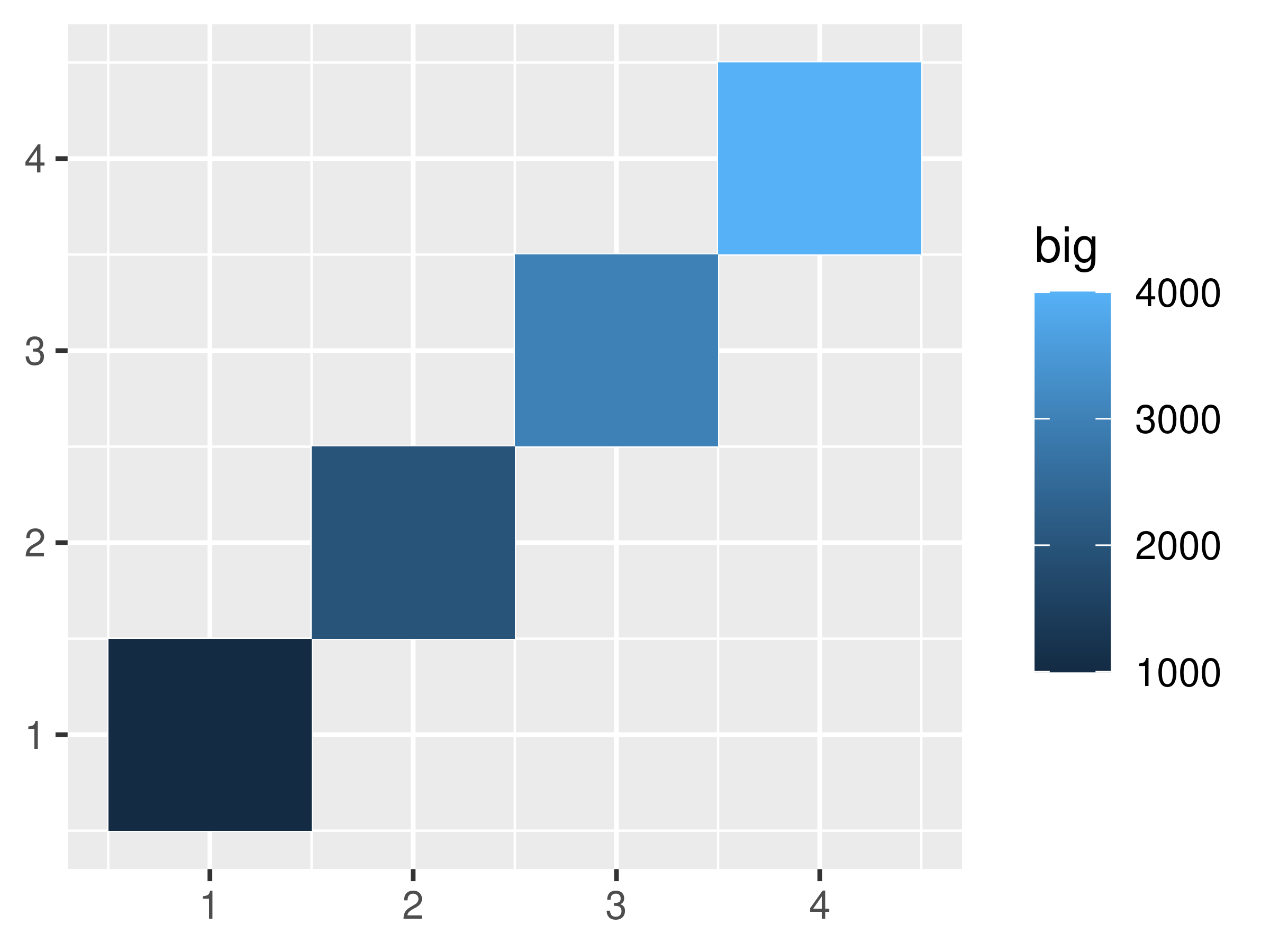
(The toy data set used here is the same one defined in Section 10.1.4). You can suppress the breaks entirely by setting them to NULL, which removes the keys and labels.
11.2.5 Legends
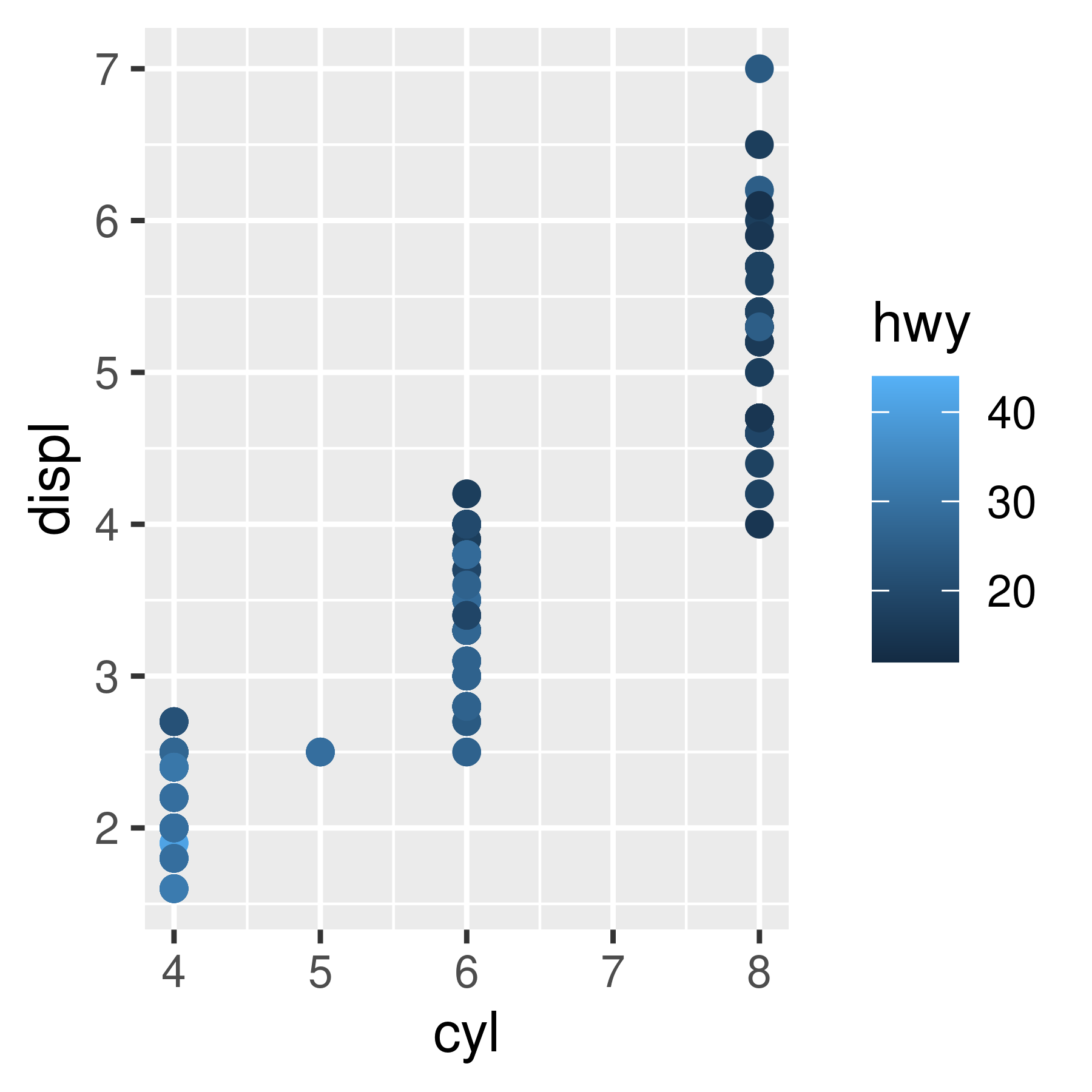
Every scale is associated with a guide that displays the relationship between the aesthetic and the data. For position scales, the axes serve this function. For colour scales this role is played by the legend, which can be customised with the help of a guide function. For continuous colour scales, the default legend takes the form of a “colour bar” displaying a continuous gradient of colours:
base <- ggplot(mpg, aes(cyl, displ, colour = hwy)) +
  geom_point(size = 2)

base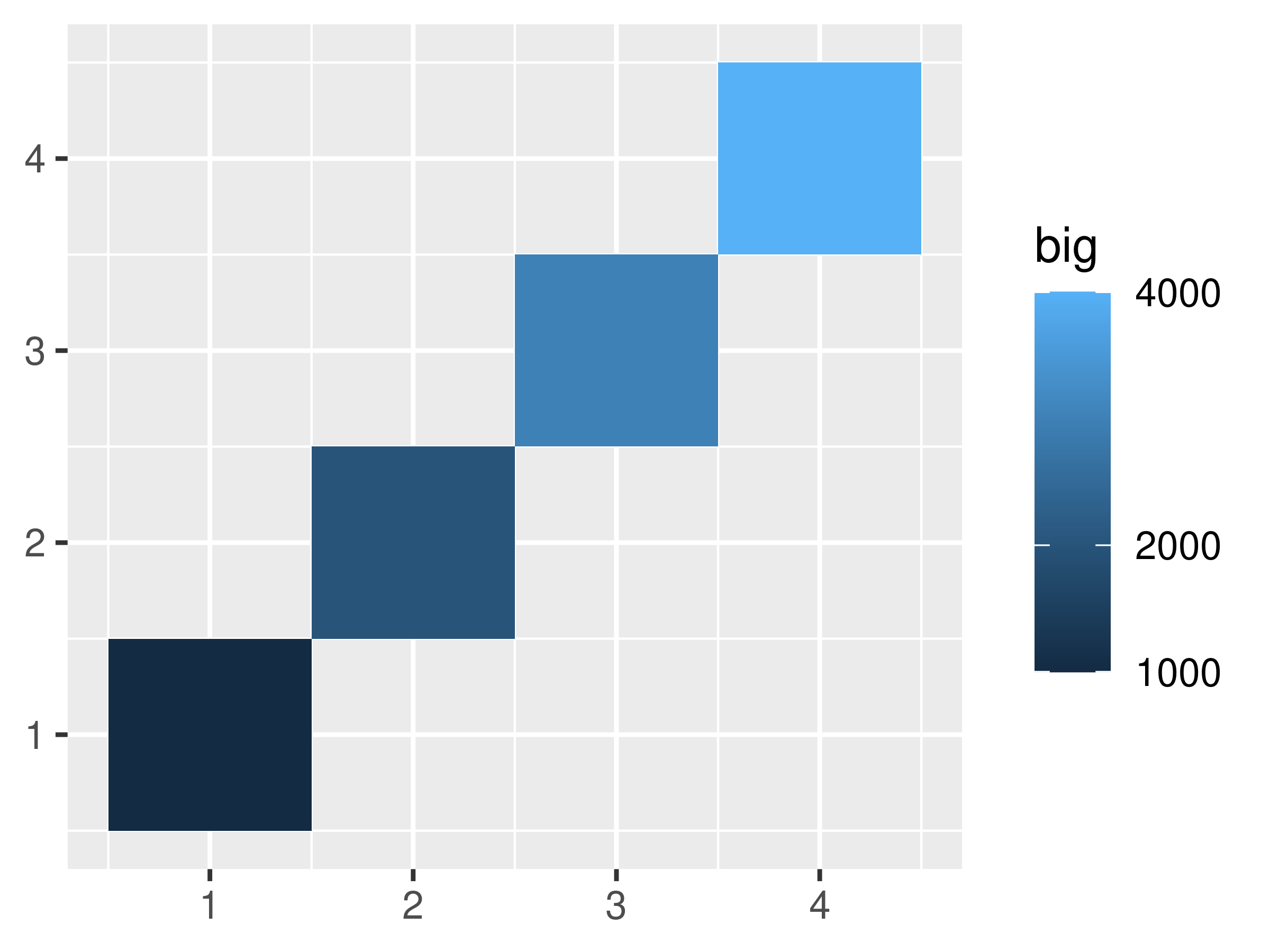
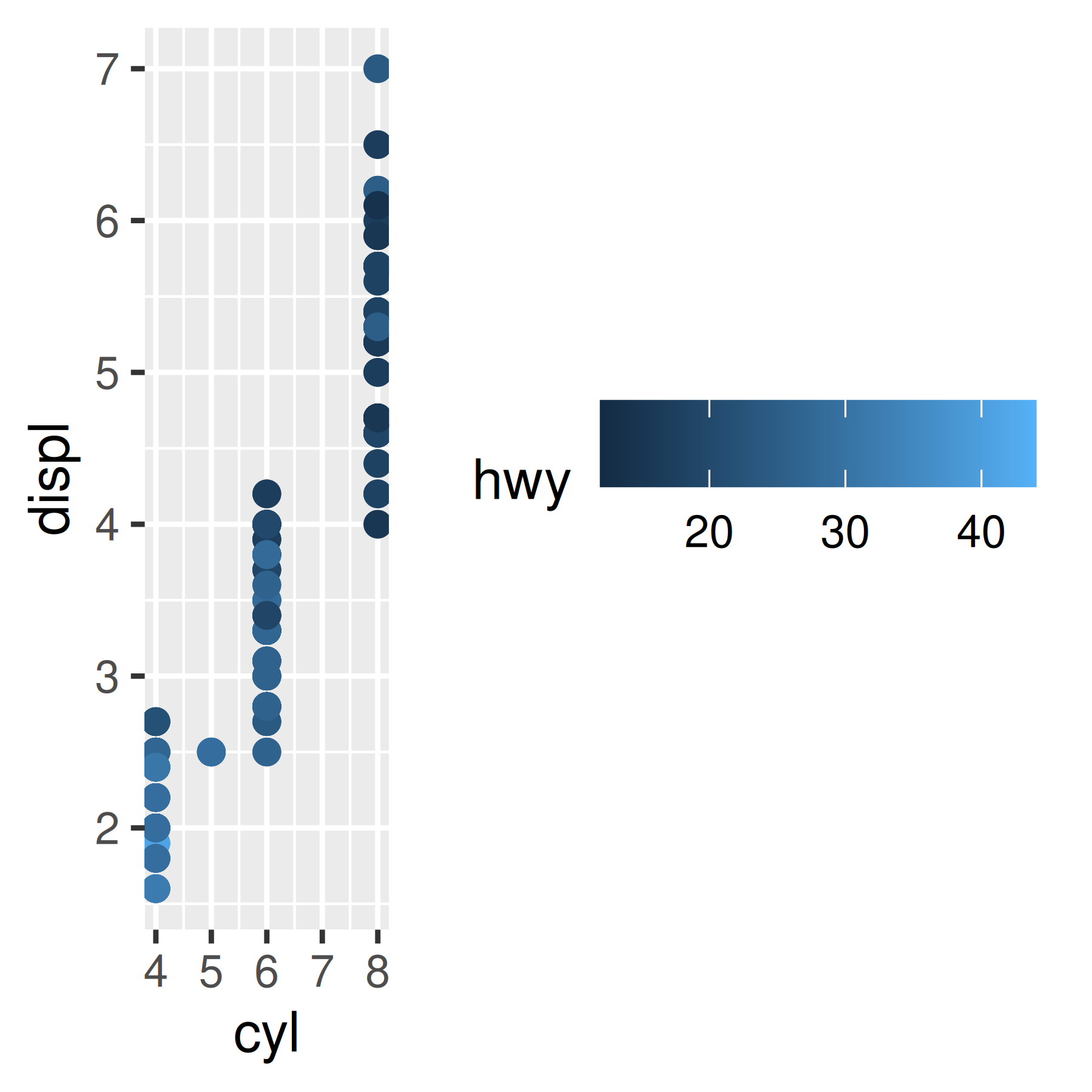
The appearance of the legend can be controlled using the guide_colourbar() function. There are many arguments to this function, allowing you to exercise precise control over the legend. The most important arguments are illustrated below:
reverseflips the colour bar to put the lowest values at the top.barwidthandbarheightallow you to specify the size of the bar. These are grid units, e.g.unit(1, "cm").directionspecifies the direction of the guide,"horizontal"or"vertical".
In Section 10.3.2 we introduced the guides() function that is used to set customised legends and axes. When applied to colour scales, it allows you to create custom legends like these:
base + guides(colour = guide_colourbar(reverse = TRUE))
base + guides(colour = guide_colourbar(barheight = unit(2, "cm")))
base + guides(colour = guide_colourbar(direction = "horizontal"))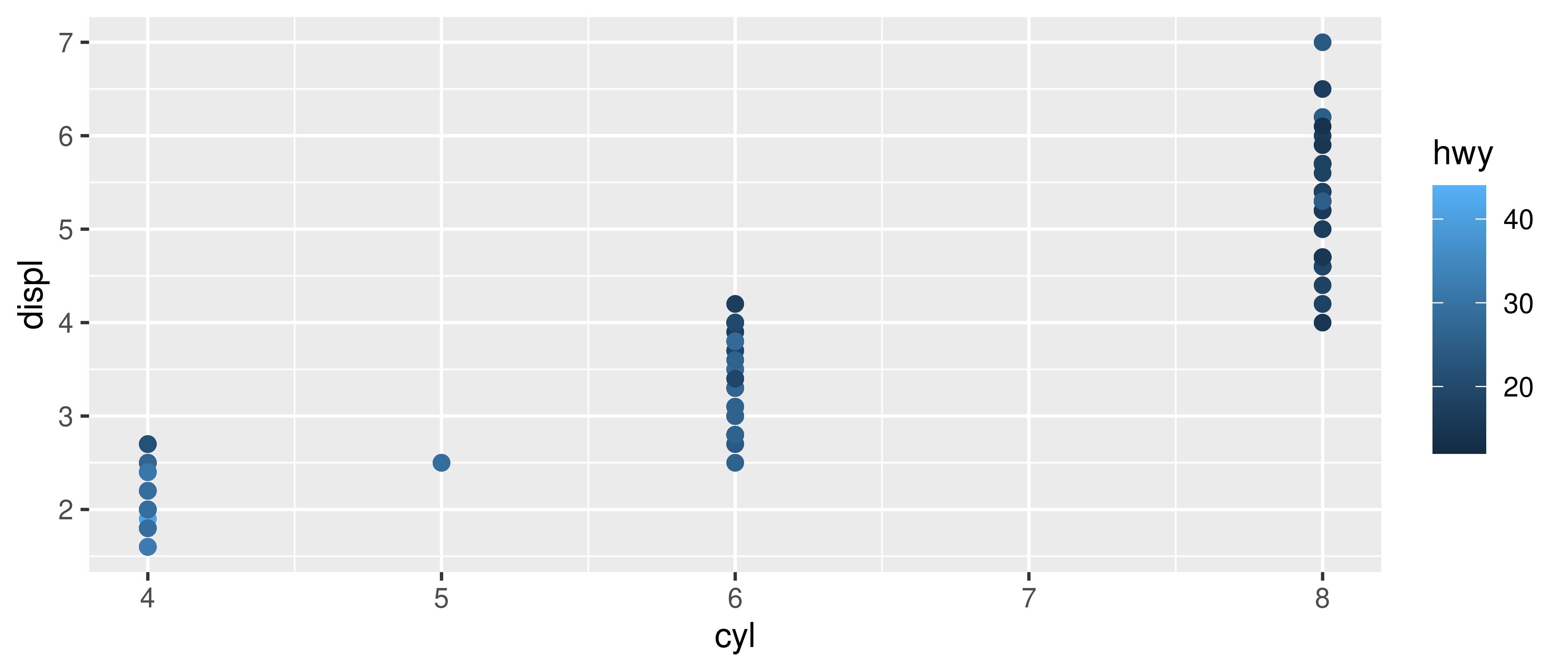

An alternative way to accomplish the same goal is to specify the guide argument to the scale function. These two plot specifications are identical:
base + guides(colour = guide_colourbar(reverse = TRUE))
base + scale_colour_continuous(guide = guide_colourbar(reverse = TRUE))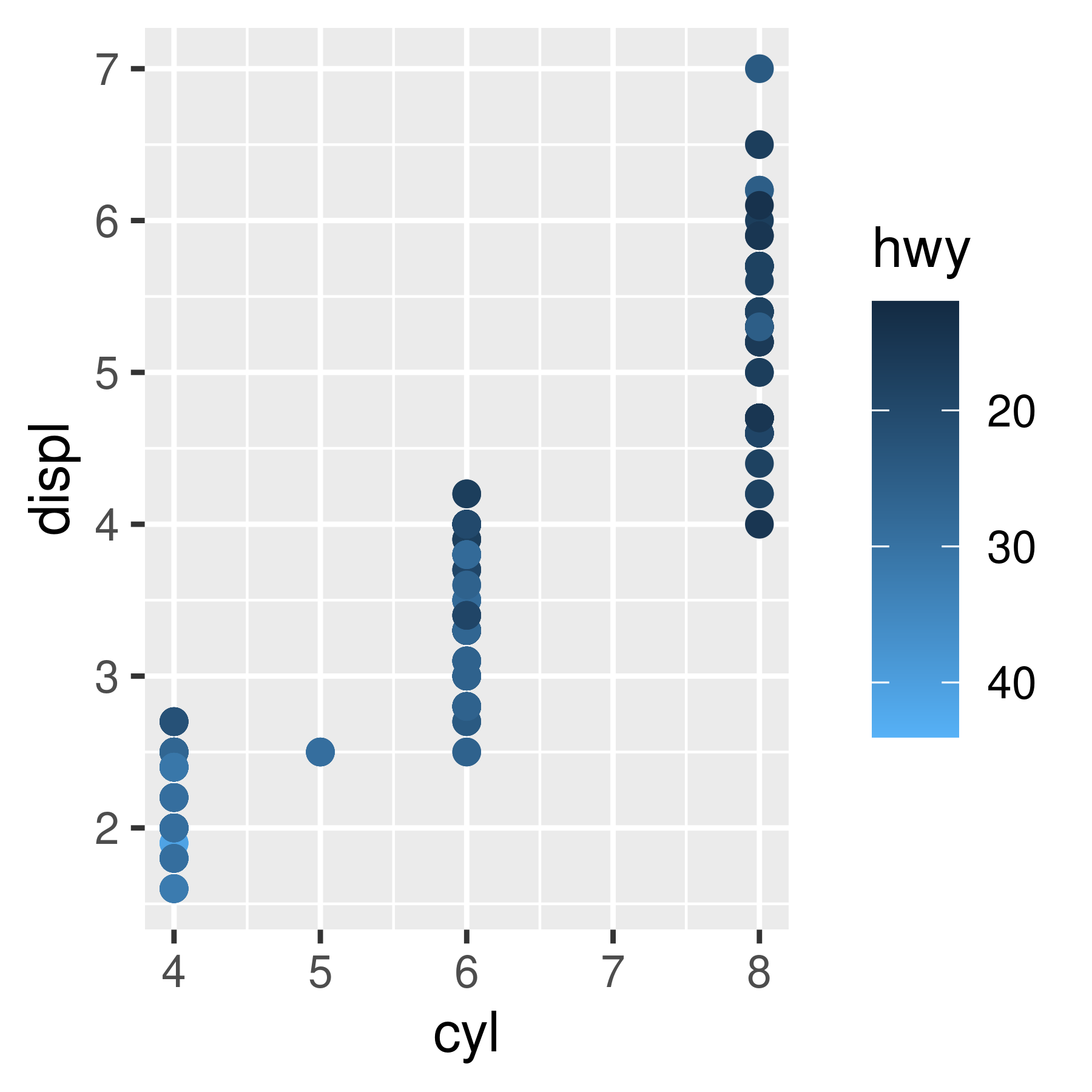
You can learn more about guide functions in Section 14.5.
11.3 Discrete colour scales
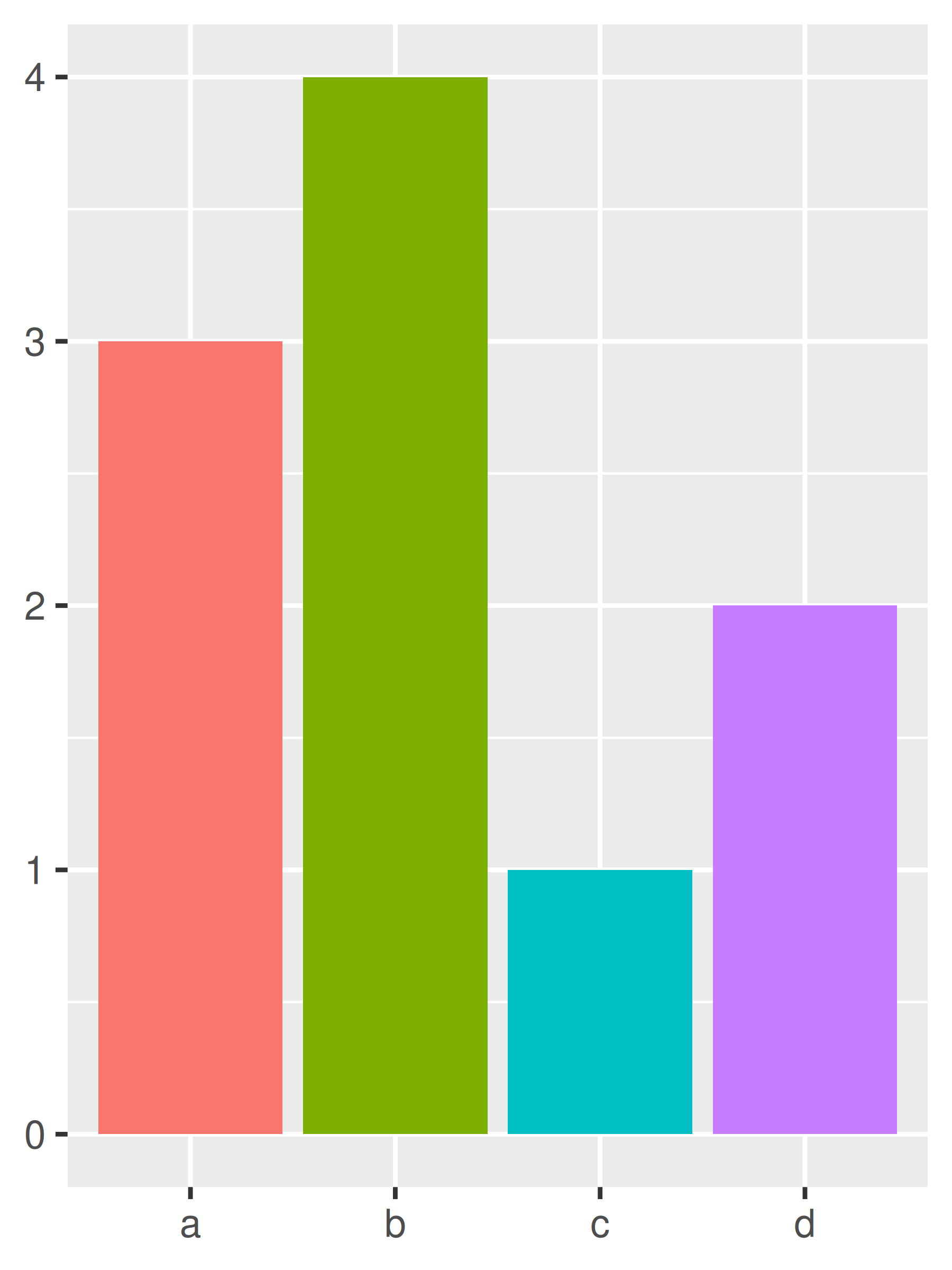
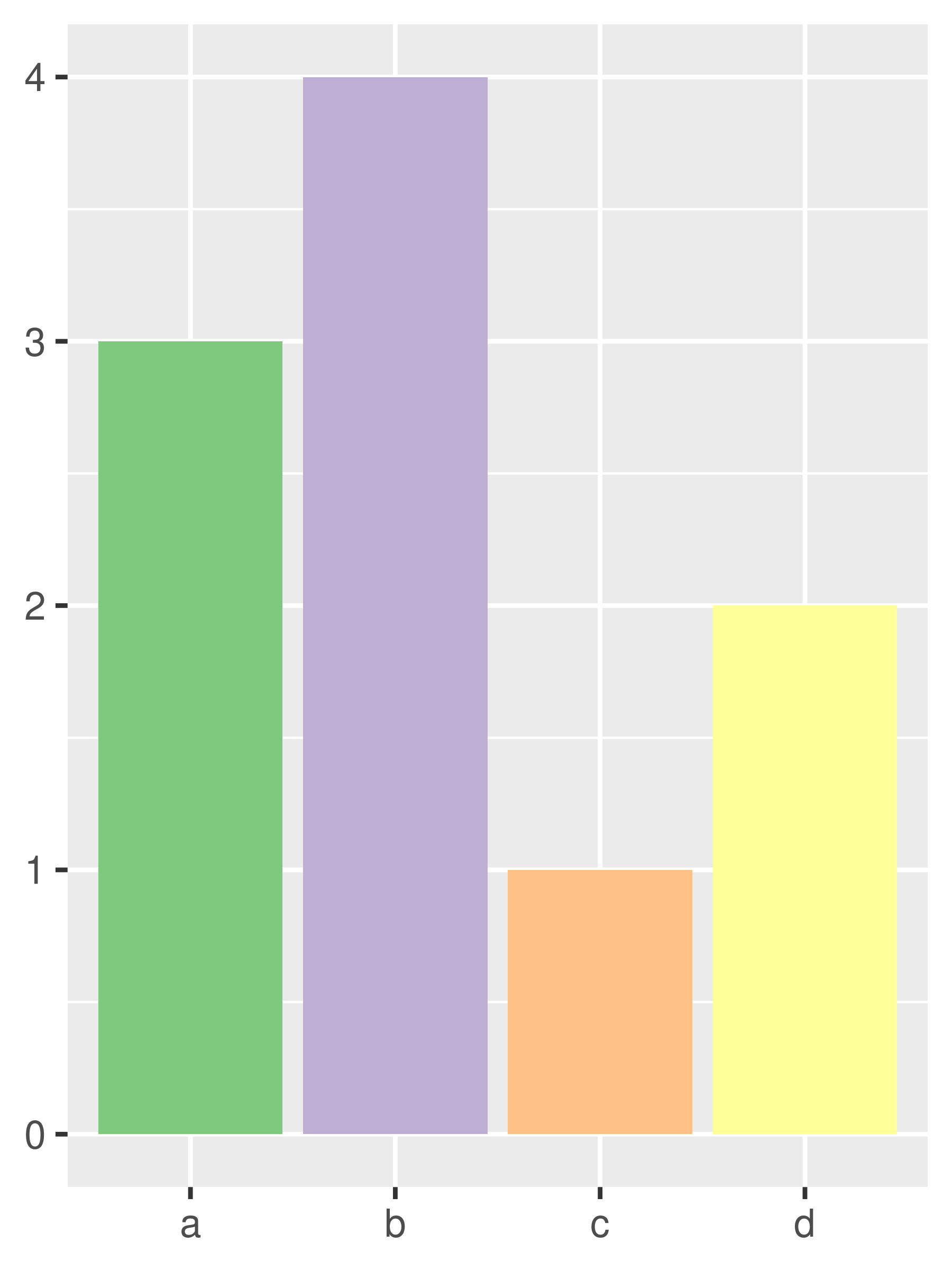
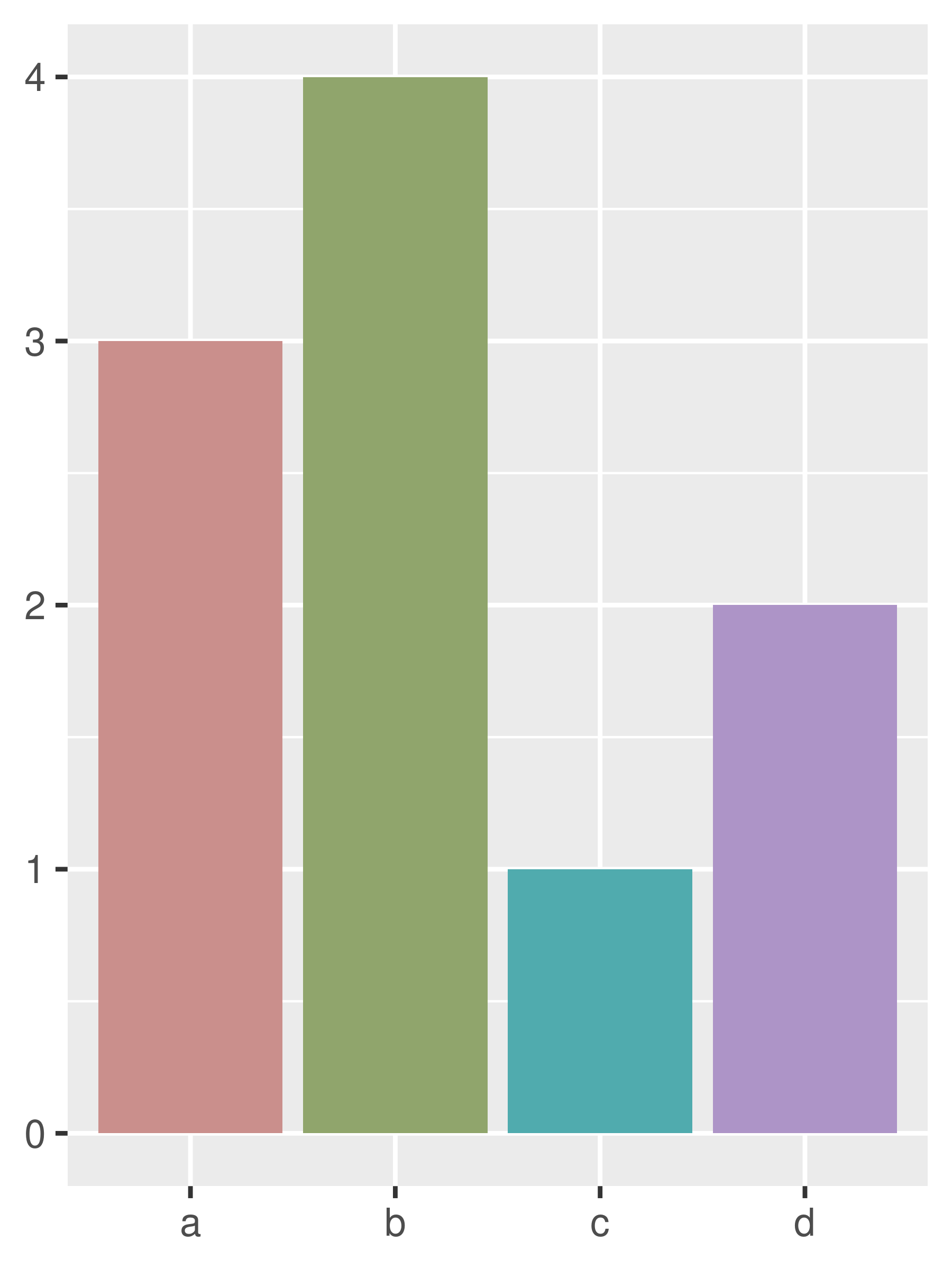
Discrete colour and fill scales occur in many situations. A typical example is a barchart that encodes both position and fill to the same variable. Many concepts from Section 11.2 apply to discrete scales, which we will illustrate using this barchart as the running example:
df <- data.frame(x = c("a", "b", "c", "d"), y = c(3, 4, 1, 2))
bars <- ggplot(df, aes(x, y, fill = x)) +
  geom_bar(stat = "identity") +
  labs(x = NULL, y = NULL) +
  theme(legend.position = "none")
The default scale for discrete colours is scale_fill_discrete() which in turn defaults to scale_fill_hue() so these are identical plots:
bars
bars + scale_fill_discrete()
bars + scale_fill_hue()

This default scale has some limitations (discussed shortly) so we’ll begin by discussing tools for producing nicer discrete palettes.
11.3.1 Brewer scales
scale_colour_brewer() is a discrete colour scale that—along with the continuous analog scale_colour_distiller() and binned analog scale_colour_fermenter()—uses handpicked “ColorBrewer” colours taken from https://colorbrewer2.org/. These colours have been designed to work well in a wide variety of situations, although the focus is on maps and so the colours tend to work better when displayed in large areas. There are many different options:
RColorBrewer::display.brewer.all()
The first group of palettes are sequential scales that are useful when your discrete scale is ordered (e.g., rank data), and are available for continuous data using scale_colour_distiller(). For unordered categorical data, the palettes of most interest are those in the second group. ‘Set1’ and ‘Dark2’ are particularly good for points, and ‘Set2’, ‘Pastel1’, ‘Pastel2’ and ‘Accent’ work well for areas.
bars + scale_fill_brewer(palette = "Set1")
bars + scale_fill_brewer(palette = "Set2")
bars + scale_fill_brewer(palette = "Accent")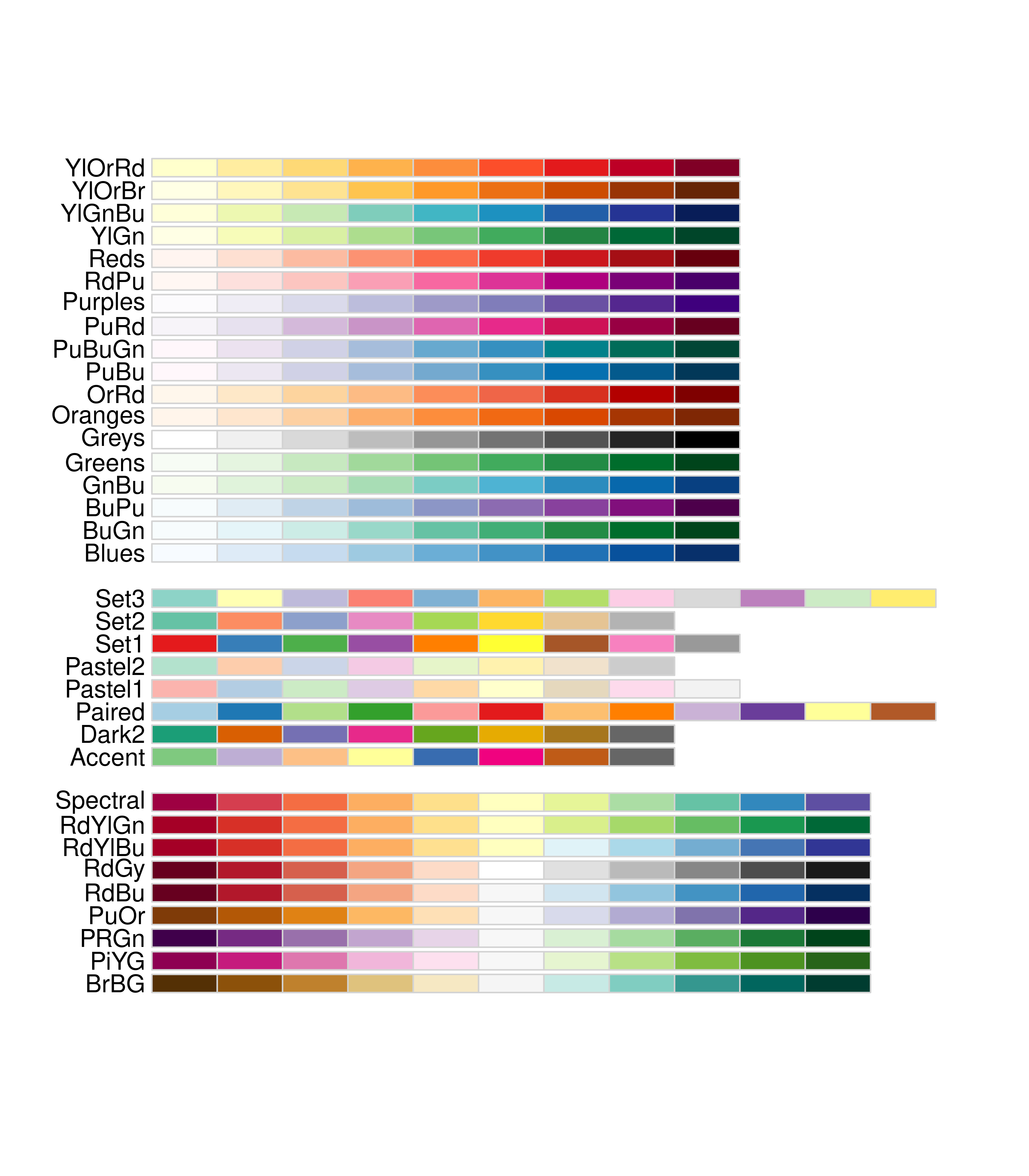


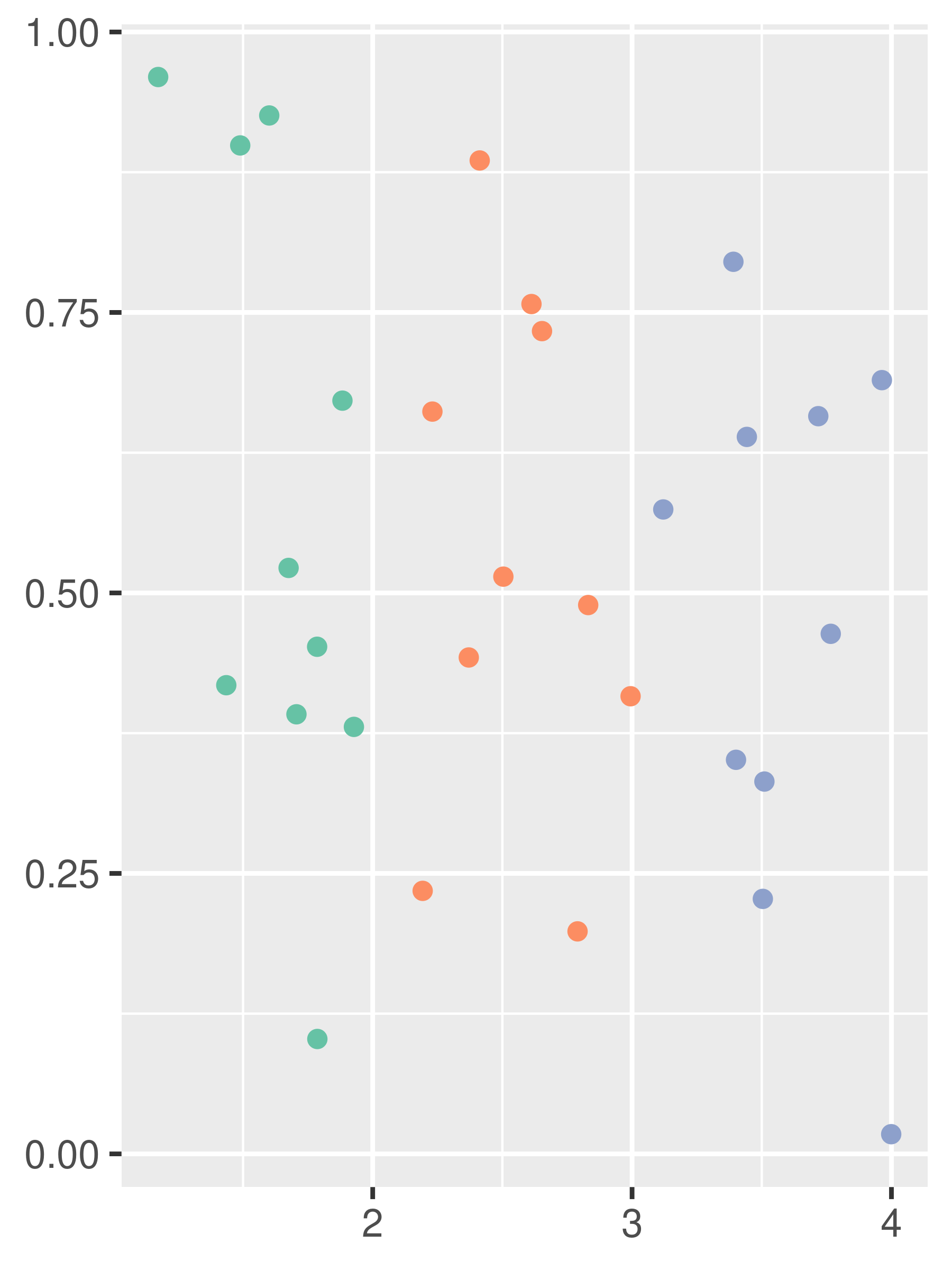
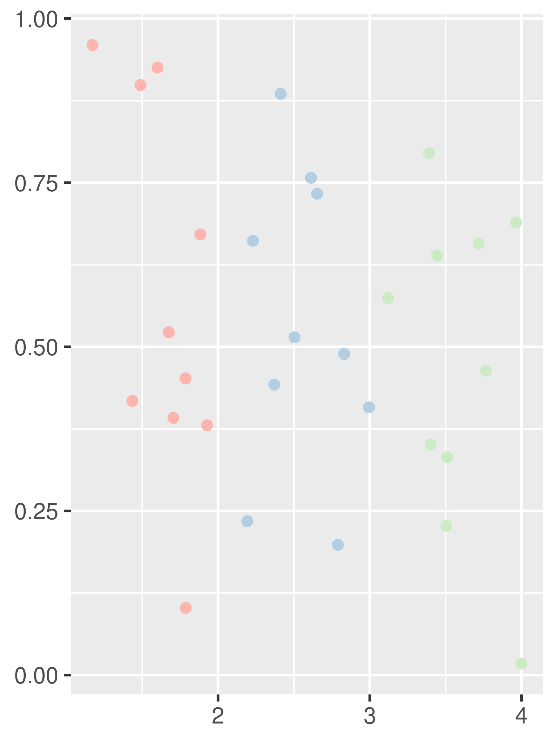
Note that no palette is uniformly good for all purposes. Scatter plots typically use small plot markers, and bright colours tend to work better than subtle ones:
# scatter plot
df <- data.frame(
  x = 1:3 + runif(30),
  y = runif(30),
  z = c("a", "b", "c")
)
point <- ggplot(df, aes(x, y)) +
  geom_point(aes(colour = z))  +
  theme(legend.position = "none") +
  labs(x = NULL, y = NULL)

# three palettes
point + scale_colour_brewer(palette = "Set1")
point + scale_colour_brewer(palette = "Set2")
point + scale_colour_brewer(palette = "Pastel1")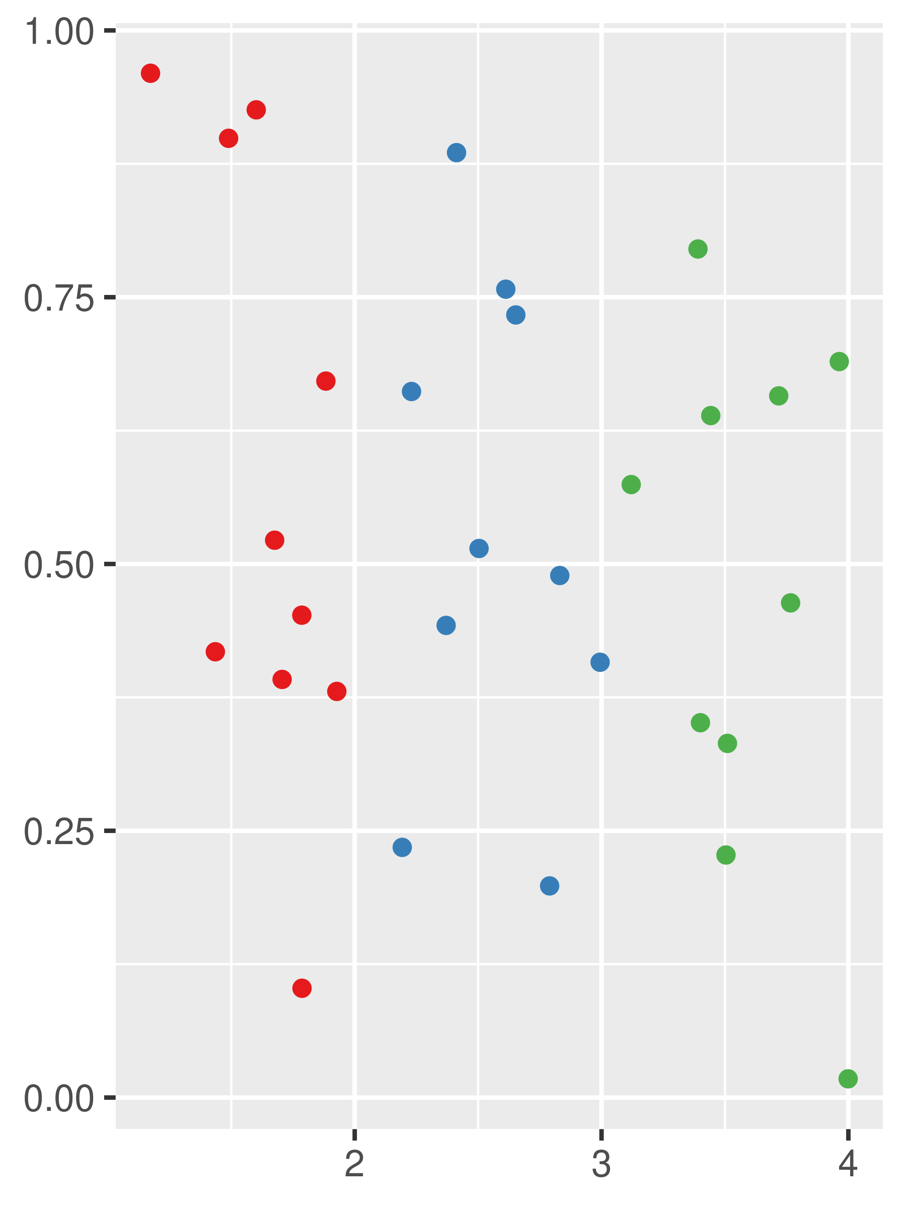
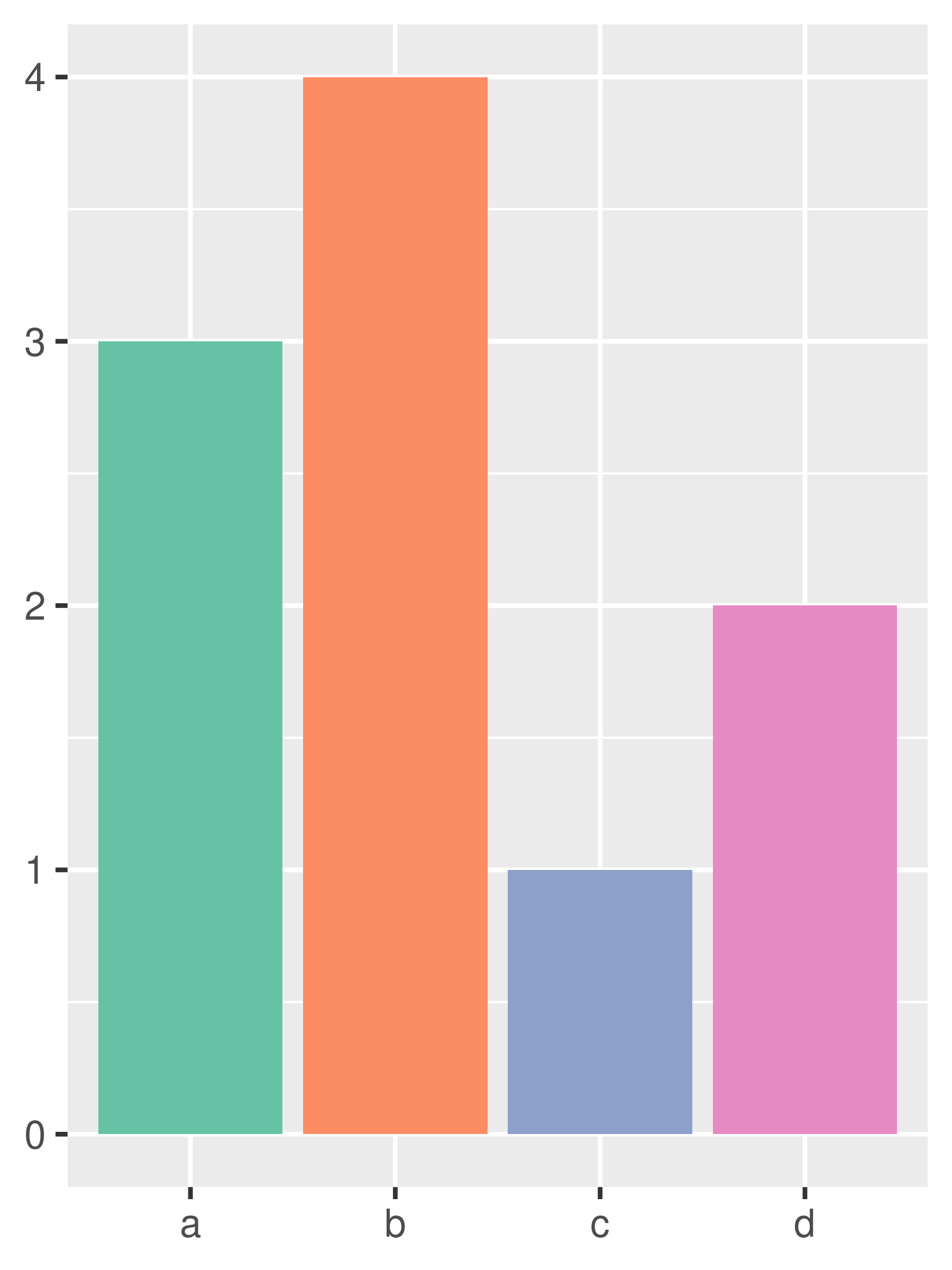
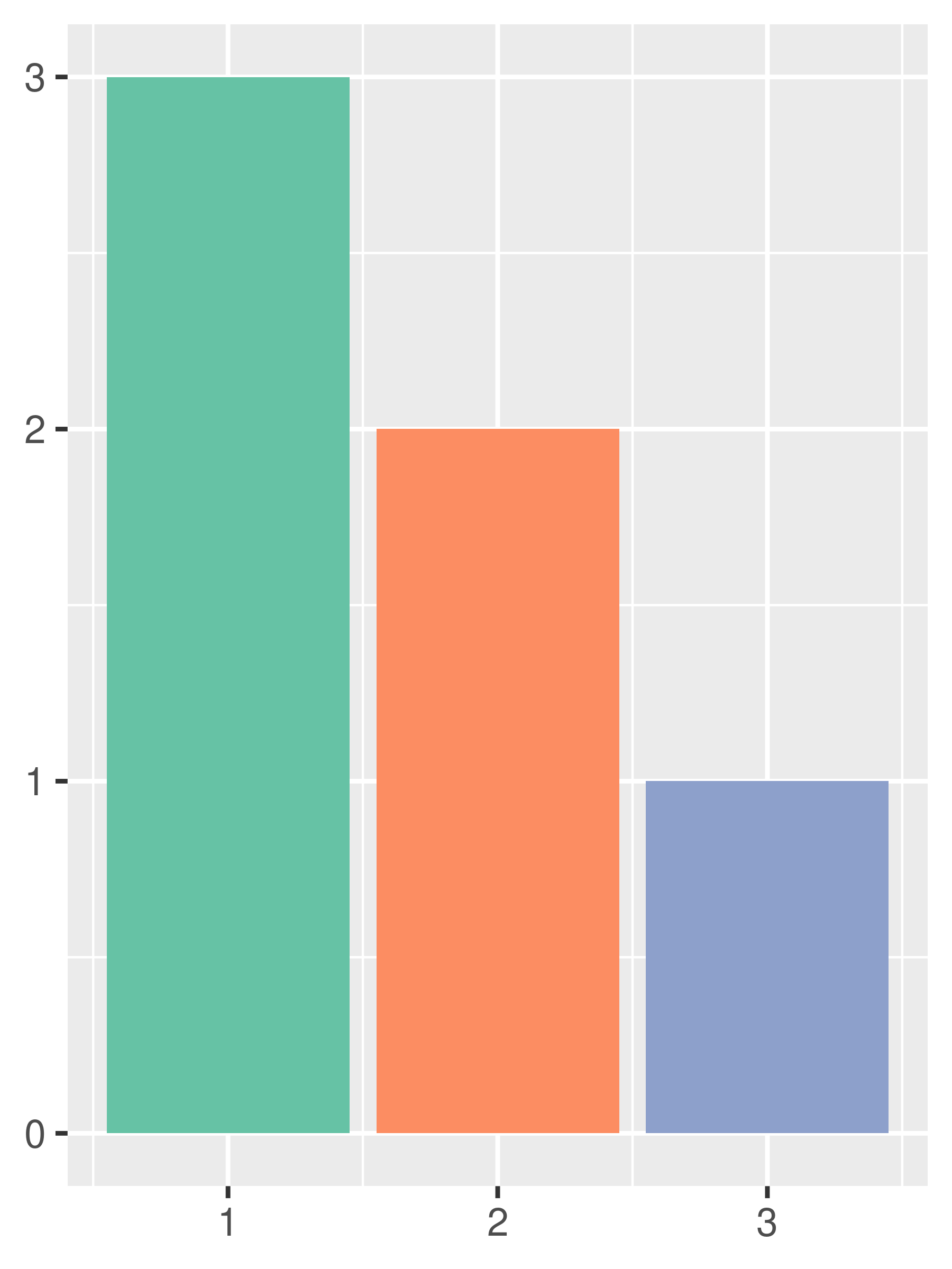
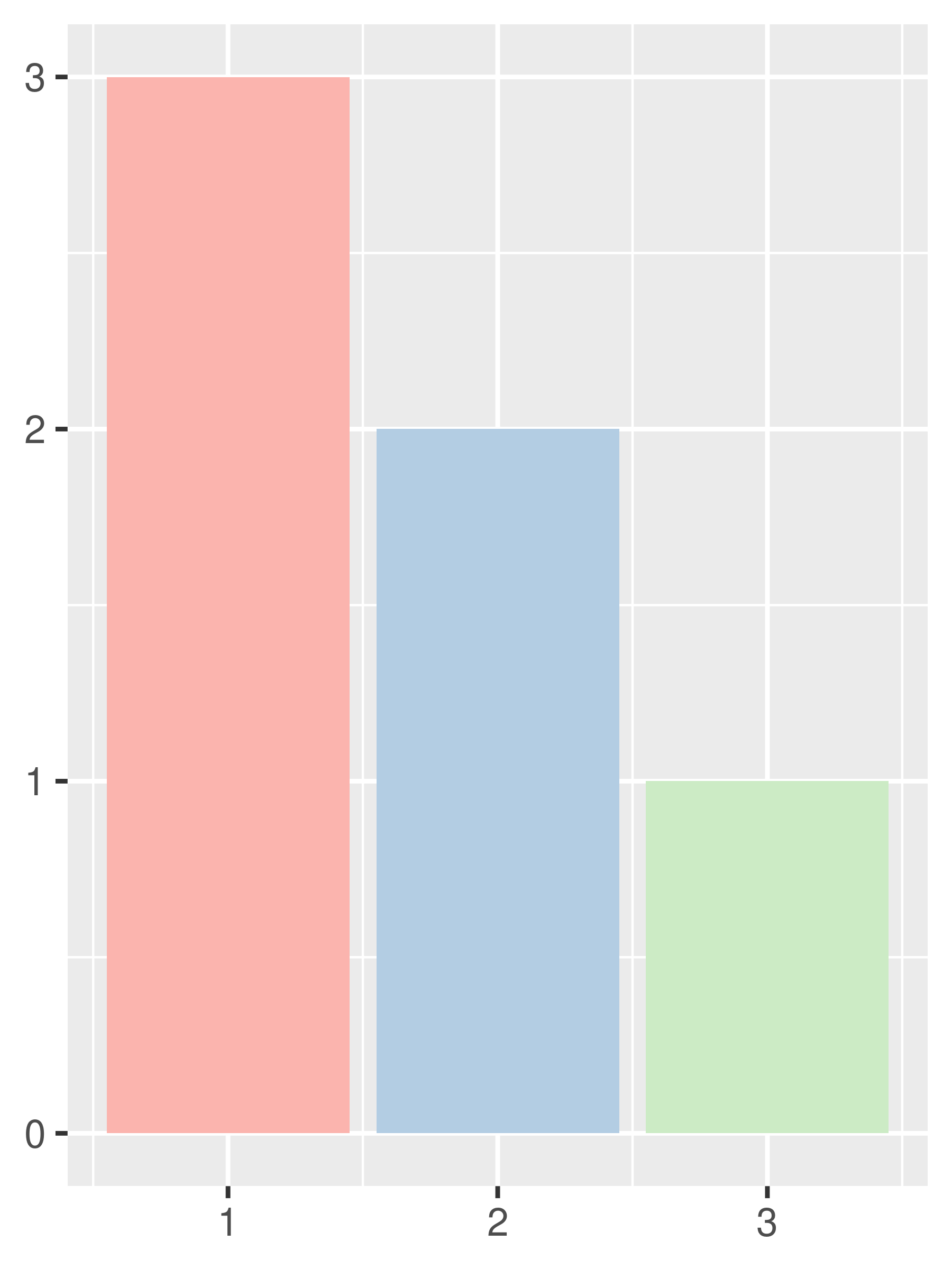
Bar plots usually contain large patches of colour, and bright colours can be overwhelming. Subtle colours tend to work better in this situation:
# bar plot
df <- data.frame(x = 1:3, y = 3:1, z = c("a", "b", "c"))
area <- ggplot(df, aes(x, y)) +
  geom_bar(aes(fill = z), stat = "identity") +
  theme(legend.position = "none") +
  labs(x = NULL, y = NULL)

# three palettes
area + scale_fill_brewer(palette = "Set1")
area + scale_fill_brewer(palette = "Set2")
area + scale_fill_brewer(palette = "Pastel1")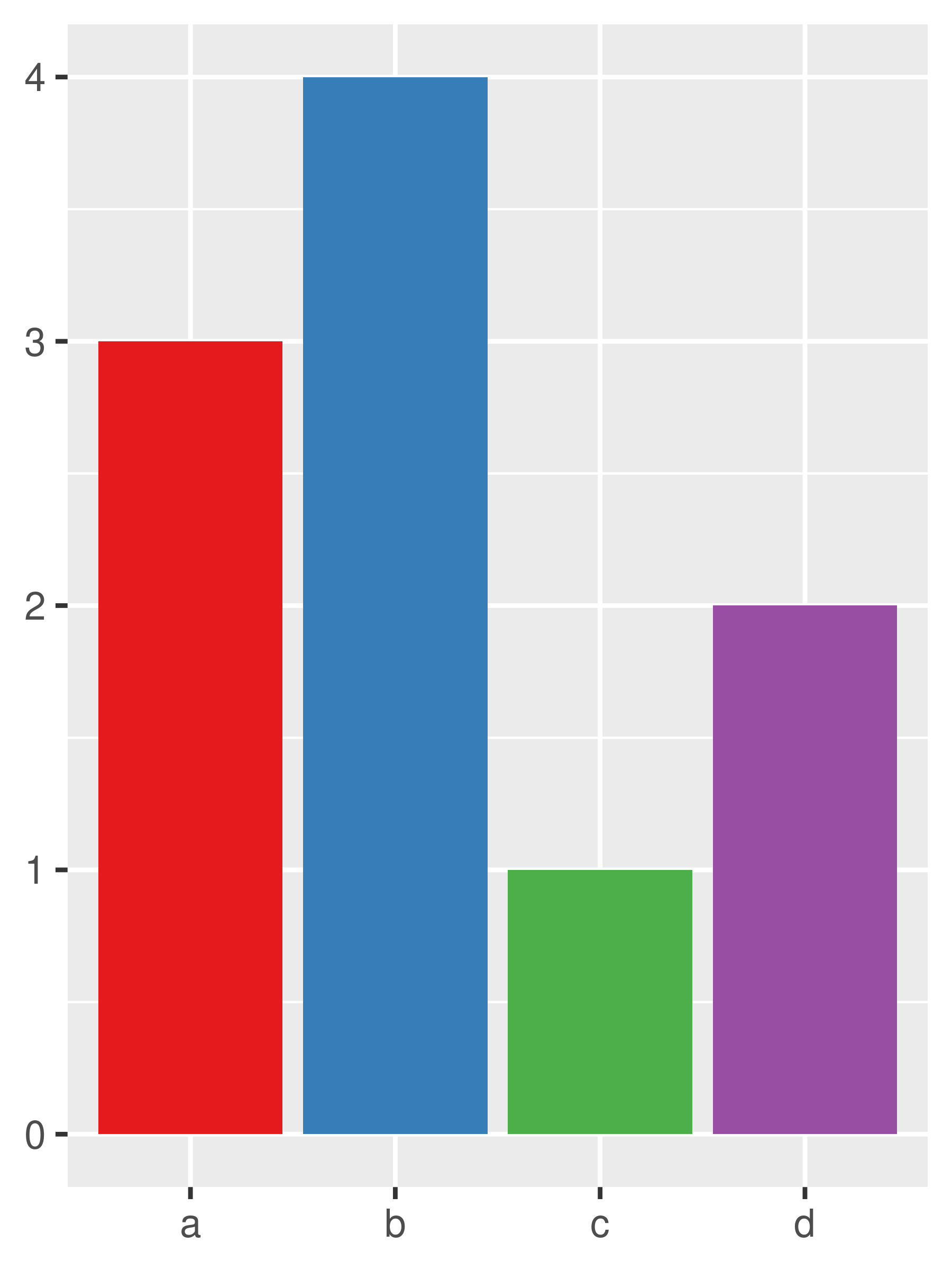
11.3.2 Hue and grey scales
The default colour scheme picks evenly spaced hues around the HCL colour wheel. This works well for up to about eight colours, but after that it becomes hard to tell the different colours apart. You can control the default chroma and luminance, and the range of hues, with the h, c and l arguments:
bars
bars + scale_fill_hue(c = 40)
bars + scale_fill_hue(h = c(180, 300))


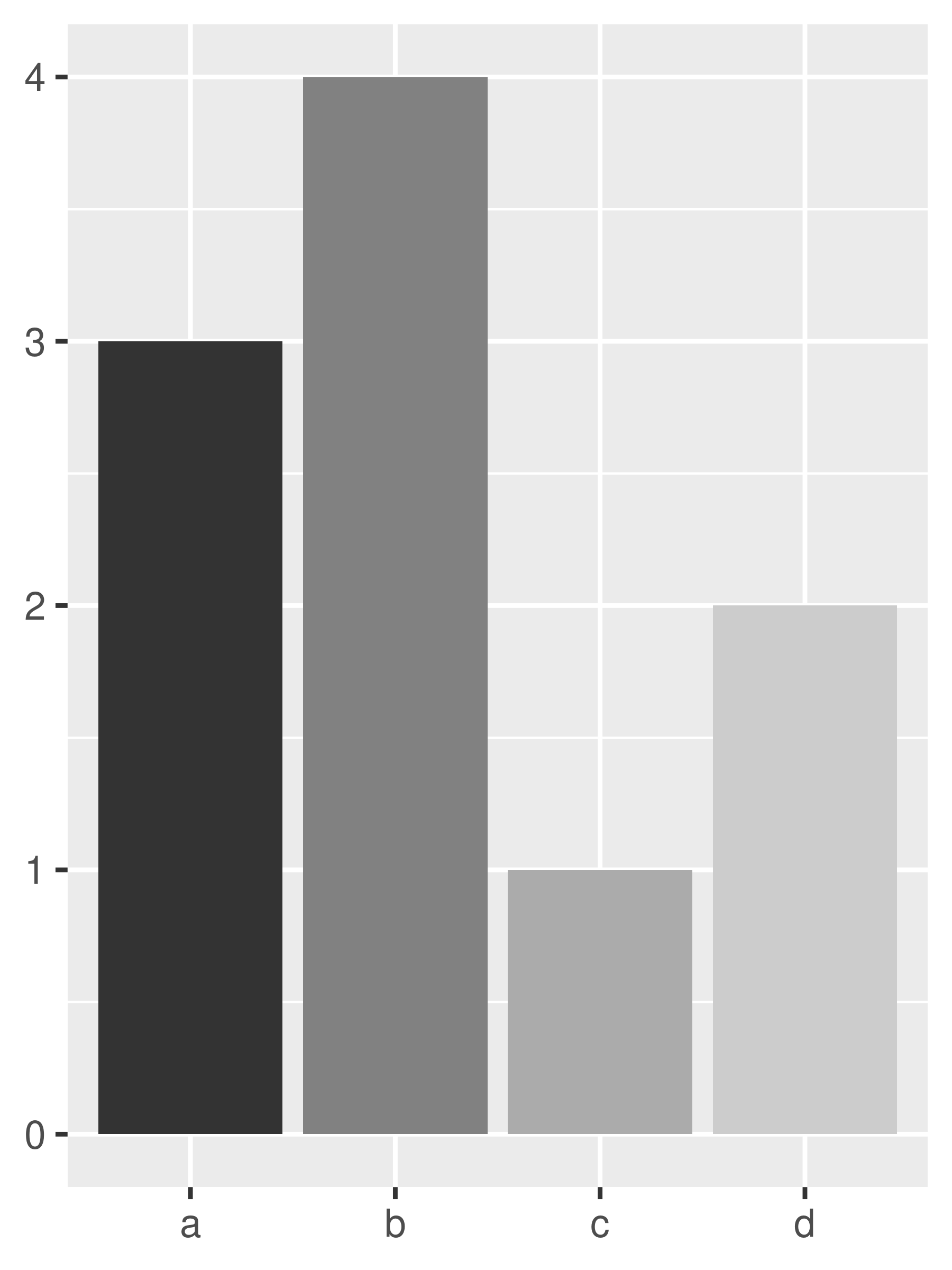
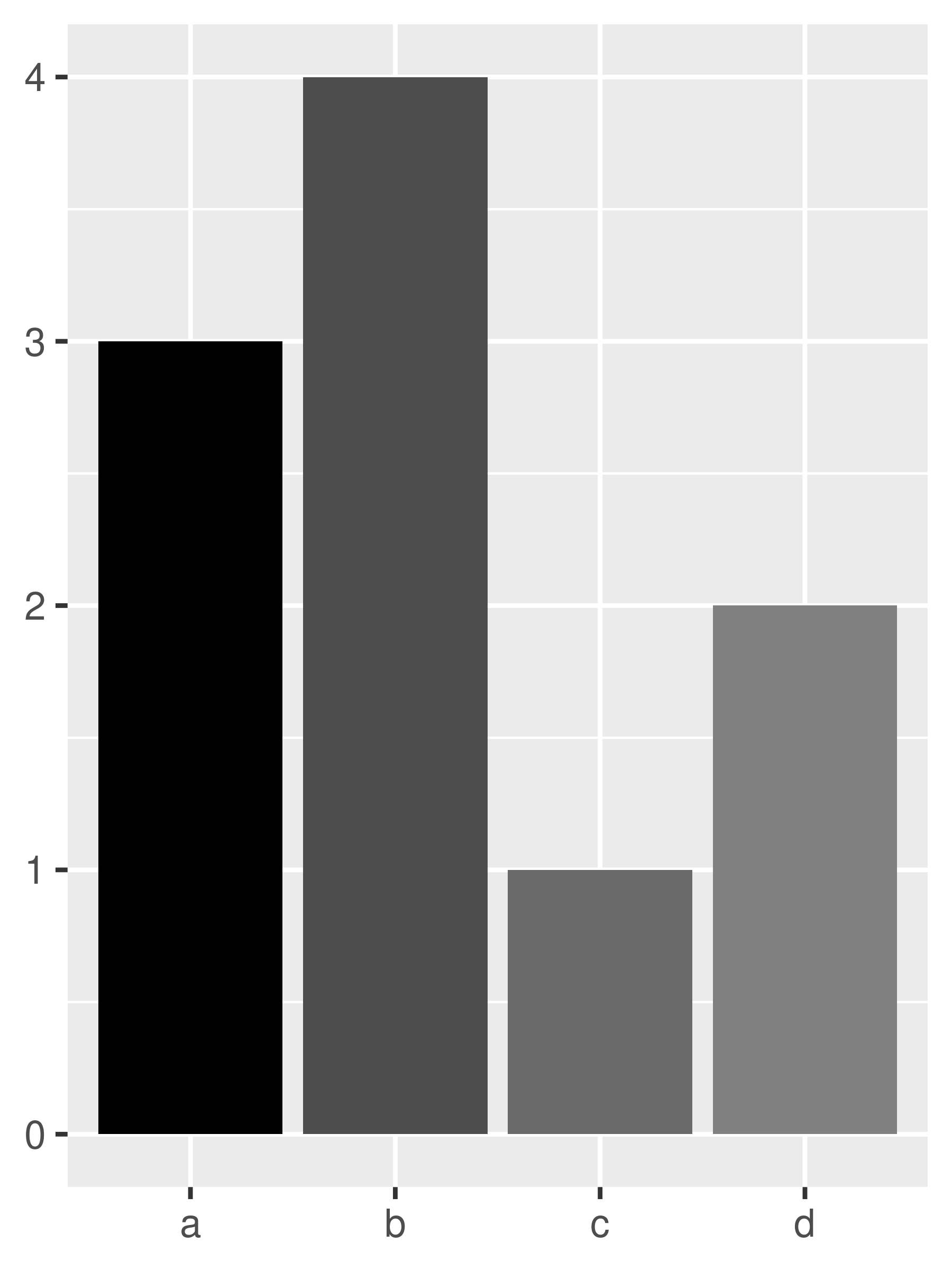
There are some problems with this default scheme. One is that unlike many of the other palettes discussed in this chapter, they are not colour blind safe (discussed in Section 11.1.1). A second is that because the colours all have the same luminance and chroma, they all appear as an identical shade of grey when printed in black and white. If you are intending a discrete colour scale to be printed in black and white, it is better to explicitly use scale_fill_grey() which maps discrete data to grays, from light to dark:
bars + scale_fill_grey()
bars + scale_fill_grey(start = 0.5, end = 1)
bars + scale_fill_grey(start = 0, end = 0.5)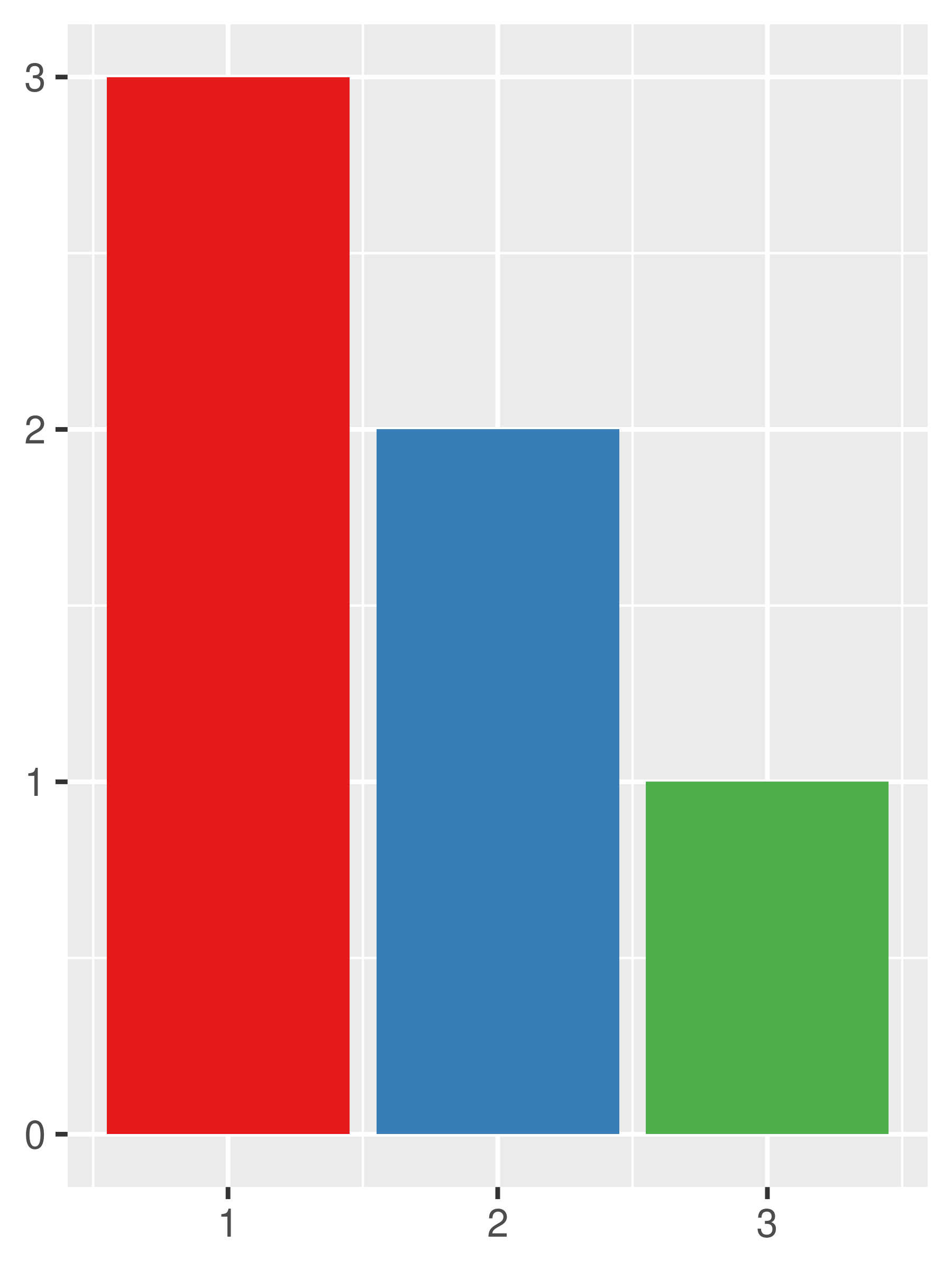
11.3.3 Paletteer scales
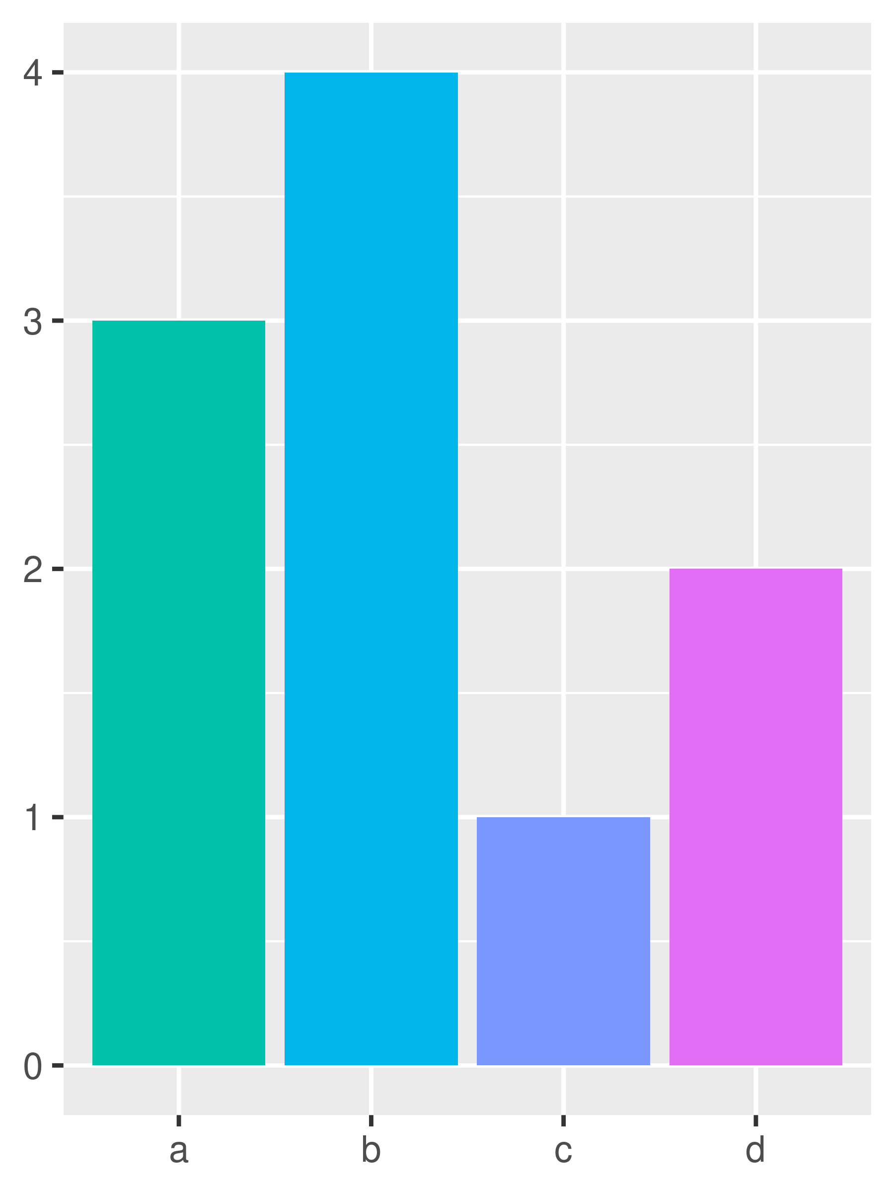
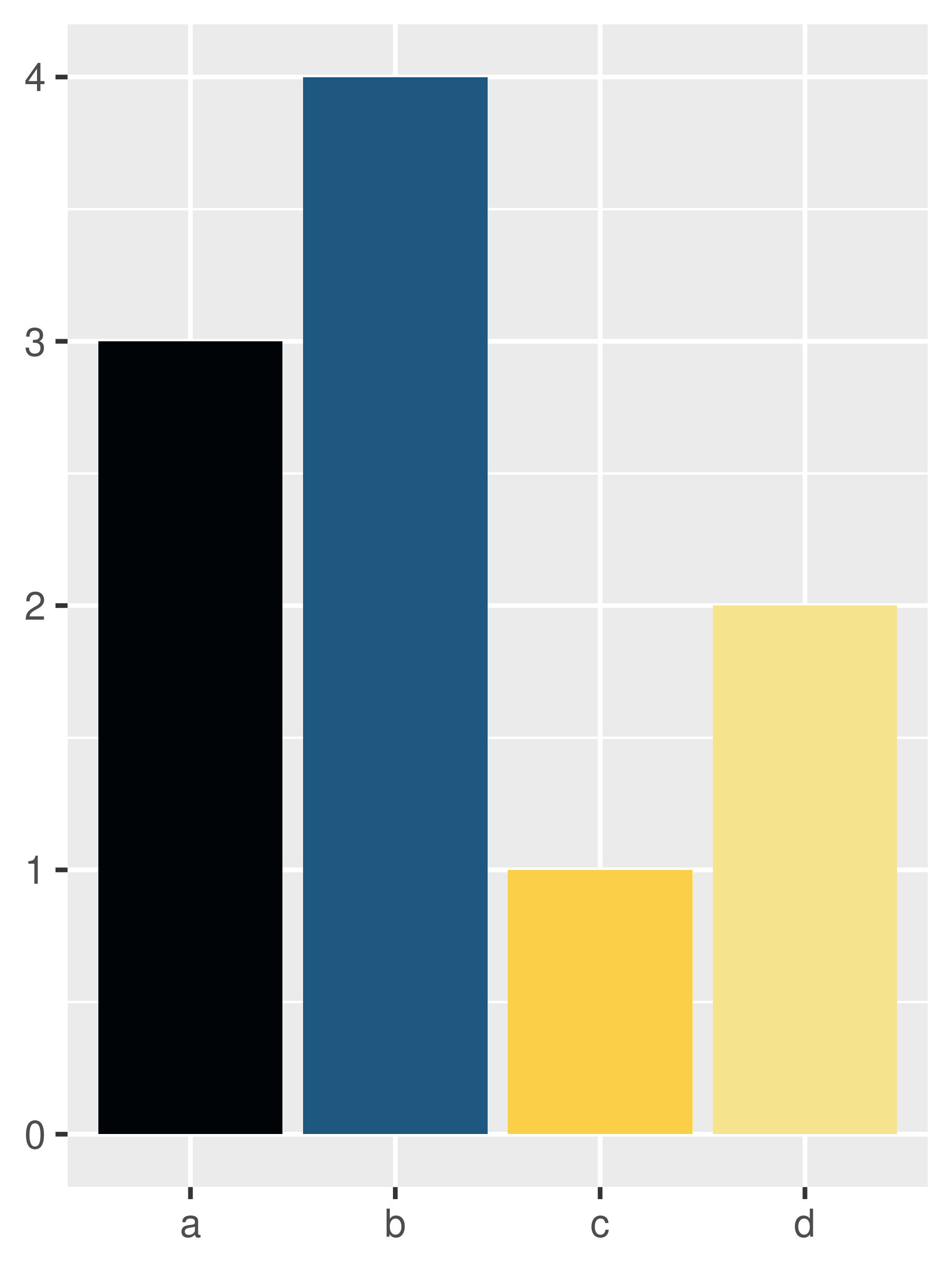
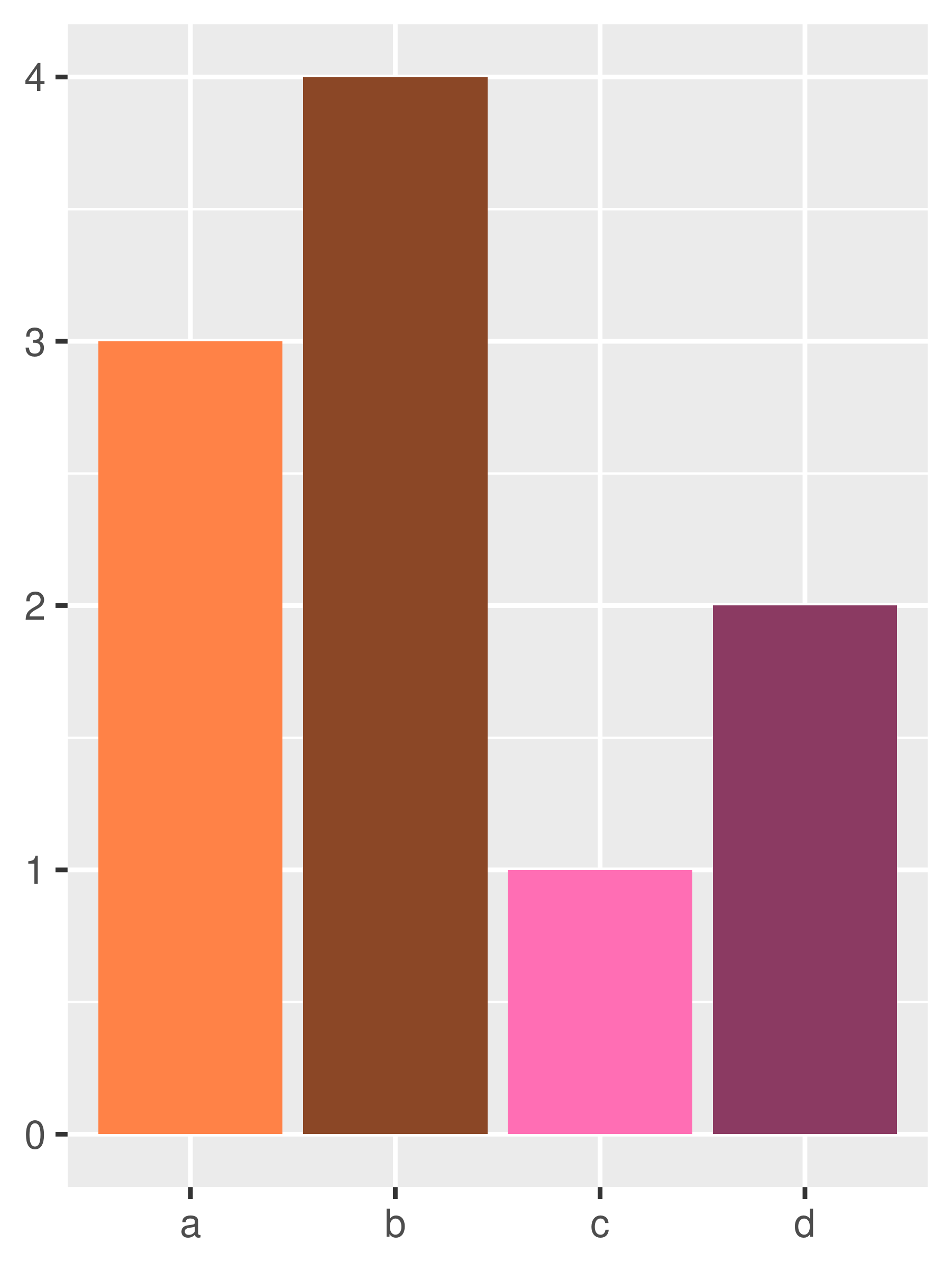
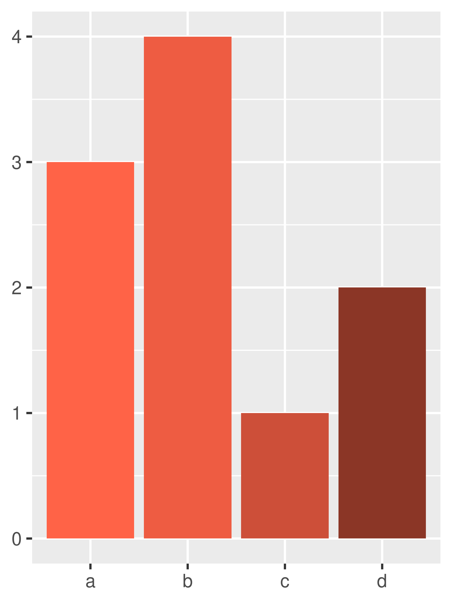
Another alternative is provided by the paletteer package, discussed earlier in connection to continuous colour scales in Section 11.2.1. By providing a unified interface that spans a large number of packages, paletteer makes it possible to choose among a very large number of palettes in a consistent way:
bars + paletteer::scale_fill_paletteer_d("rtist::vangogh")
bars + paletteer::scale_fill_paletteer_d("colorBlindness::paletteMartin")
bars + paletteer::scale_fill_paletteer_d("wesanderson::FantasticFox1")
11.3.4 Manual scales
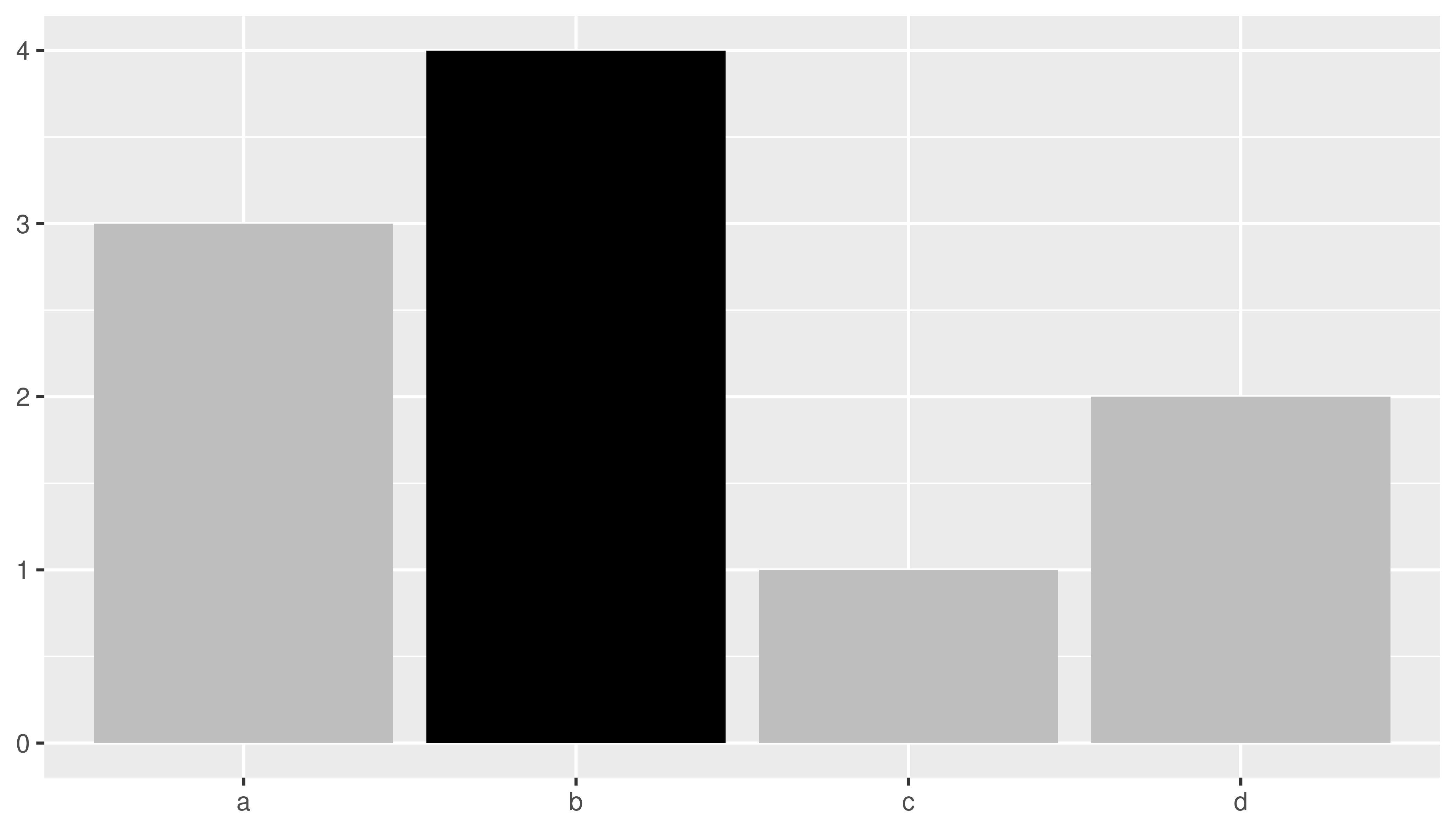
If none of the preexisting palettes is suitable, or if you have your own preferred colours, you can use scale_fill_manual() to set the colours manually. This can be useful if you wish to choose colours that highlight a secondary grouping structure or draw attention to different comparisons:
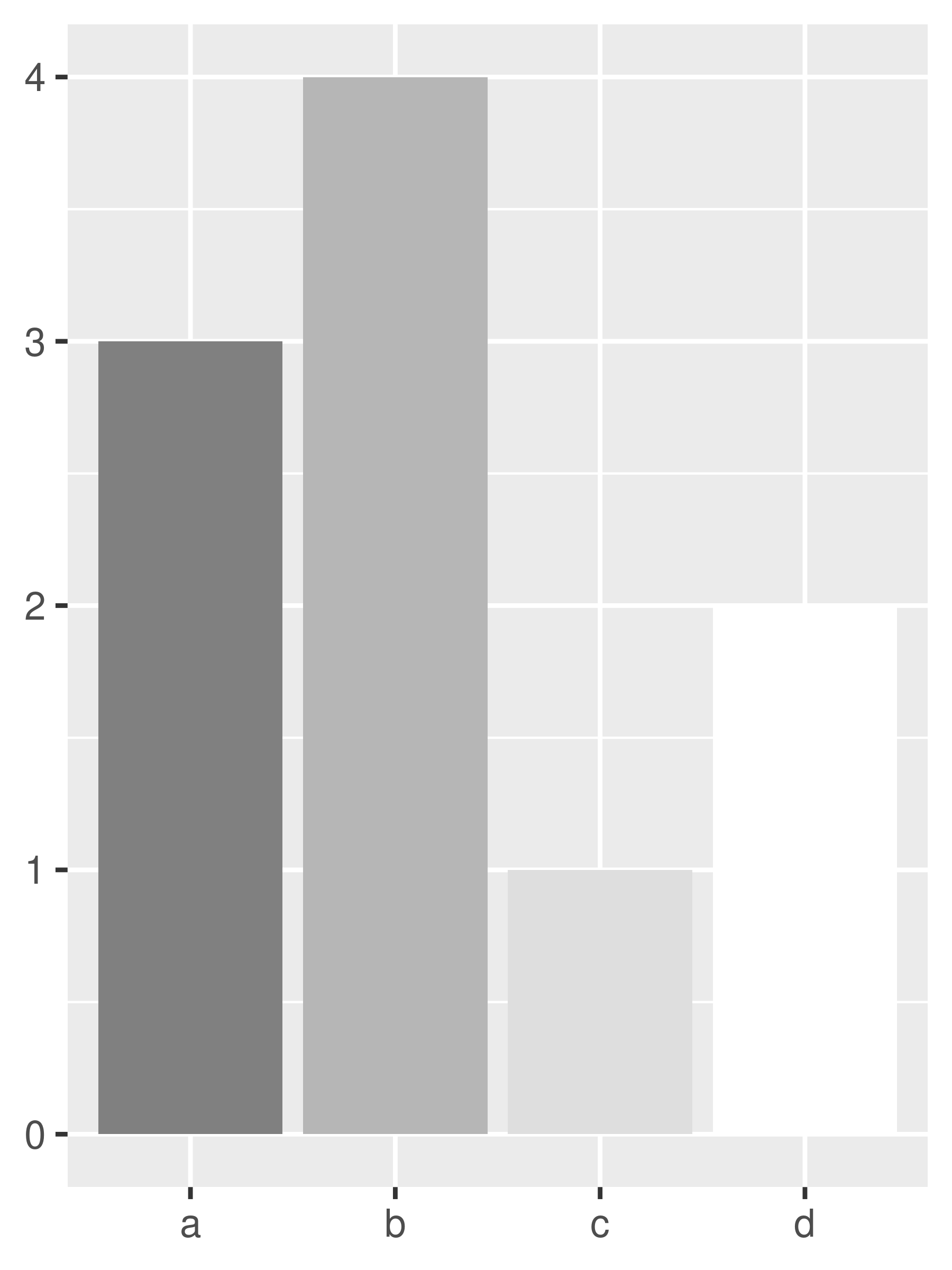
You can also use a named vector to specify colors to be assigned to each level which allows you to specify the levels in any order you like:
bars +
  scale_fill_manual(
    values = c(
      "d" = "grey",
      "c" = "grey",
      "b" = "black",
      "a" = "grey"
    )
  )
For more information about manual scales see Section 12.5.
11.3.5 Limits, breaks, and labels
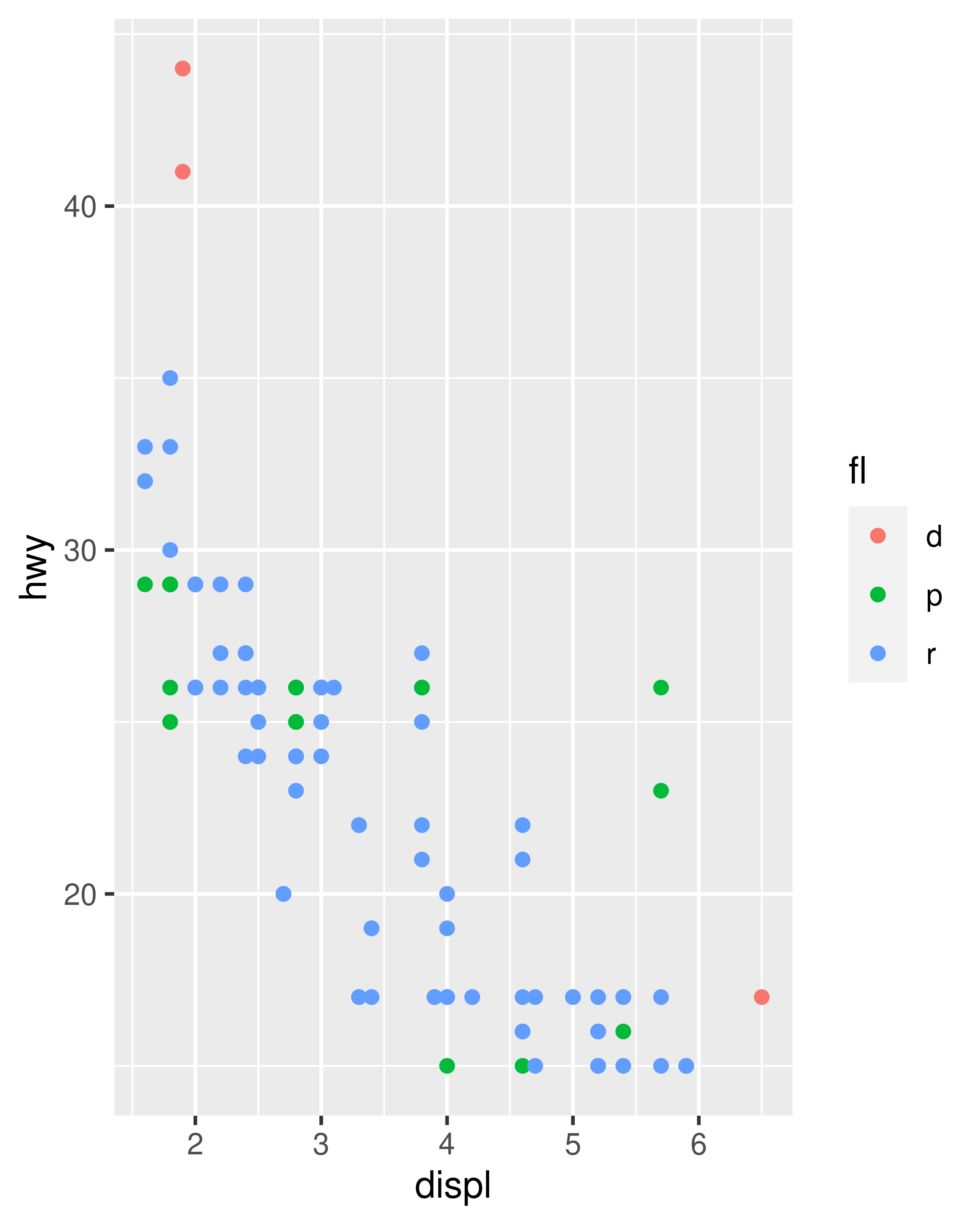
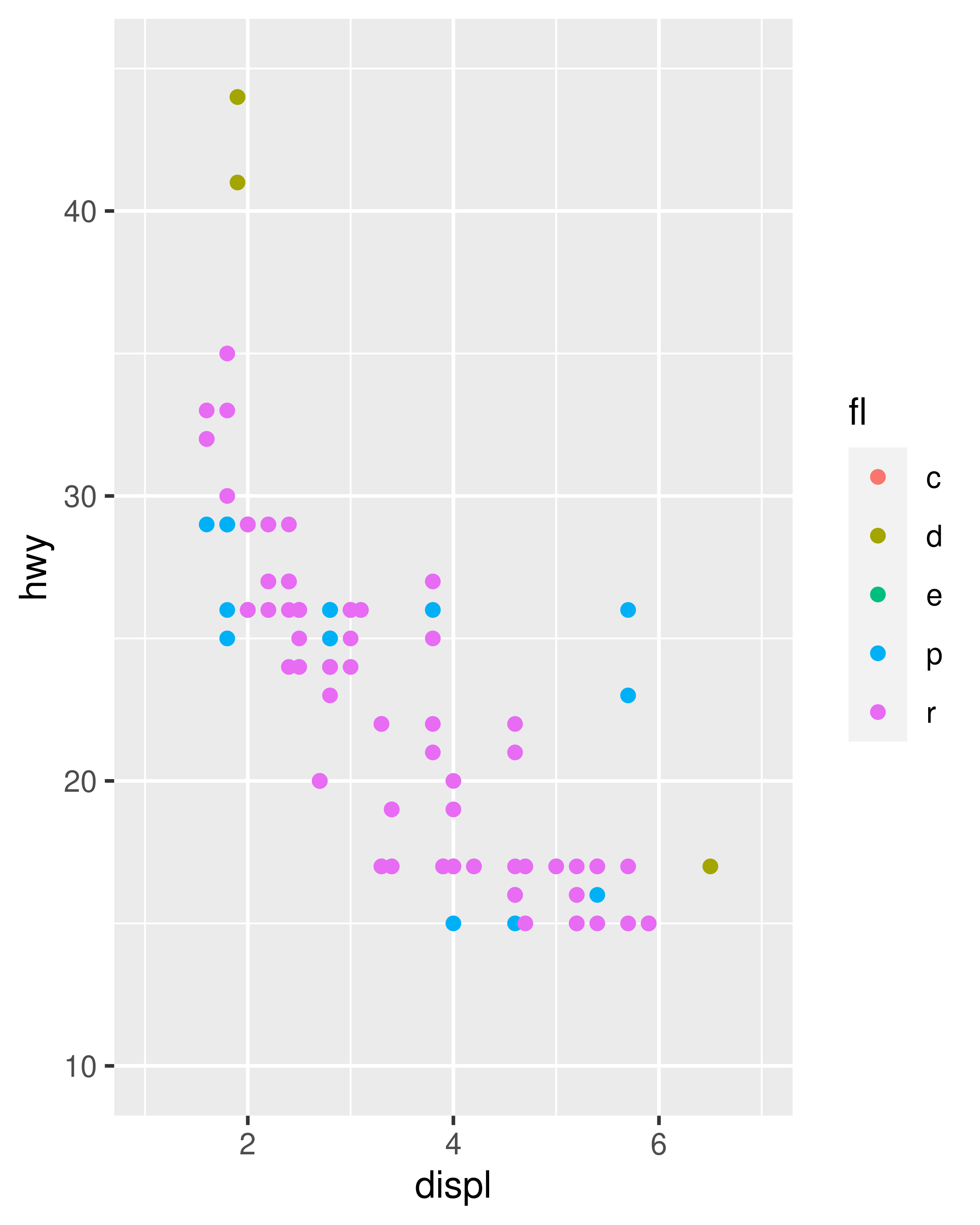
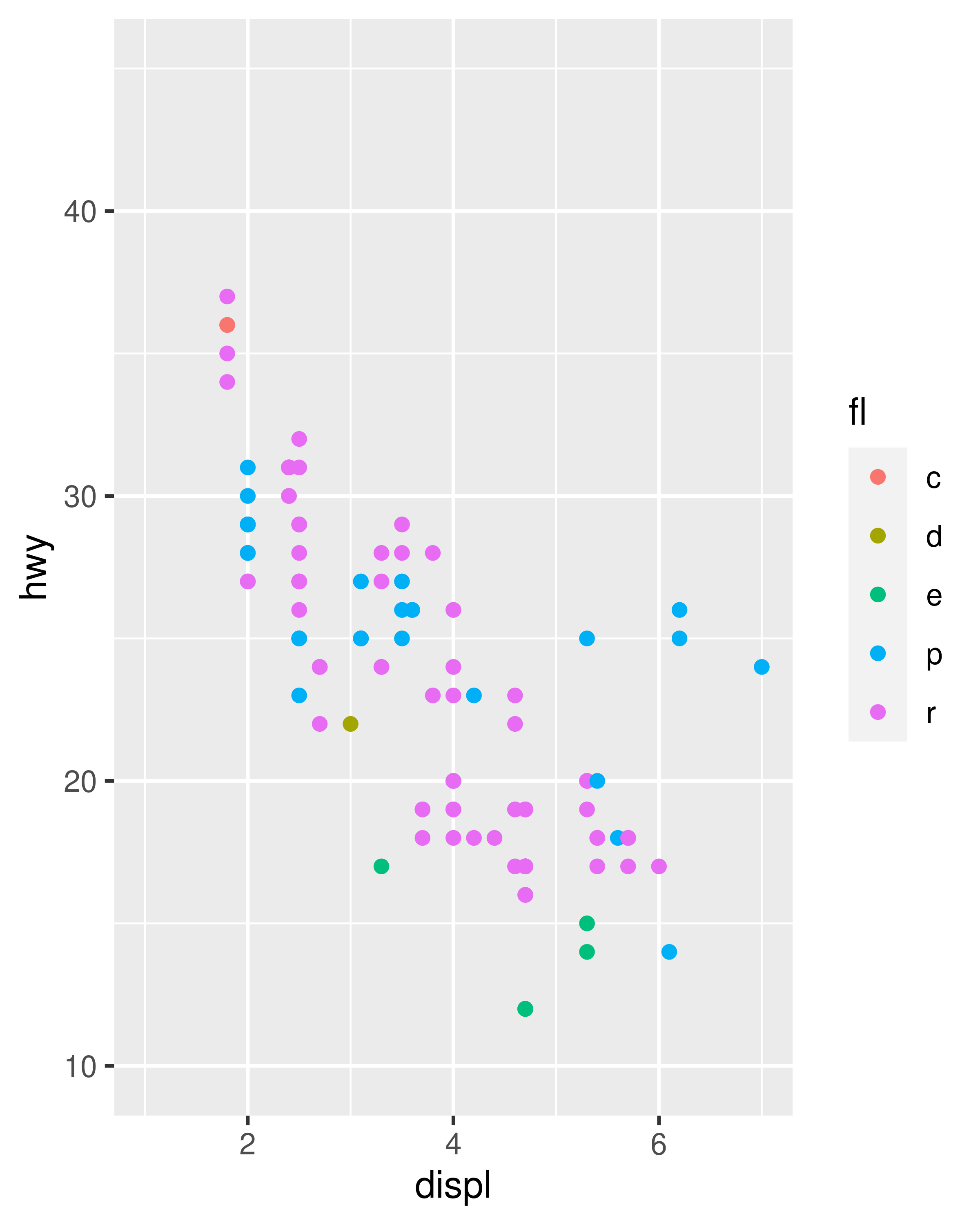
Scale limits for discrete colour scales can be set using the limits argument to the scale argument, or by using the lims() helper function. This can be important when the same variable is represented in different plots, and you want to ensure that the colours are consistent across plots. To demonstrate this, we’ll extend the example from Section 10.1.1. Colour represents the fuel type, which can be regular, ethanol, diesel, premium or compressed natural gas.
Each plot makes sense on its own, but visual comparison between the two is difficult. The axis limits are different, and because only regular, premium and diesel fuels are represented in the 1998 data the colours are mapped inconsistently. To ensure a consistent mapping for the colour aesthetic, we can use lims() to manually set the limits. As discussed in Section 10.1.1 it takes name-value pairs as input, where the name specifies the aesthetic and the value specifies the limits:

The nice thing about lims() is that we can set the limits for multiple aesthetics at once. To ensure that x, y, and colour all use consistent limits we can do this:
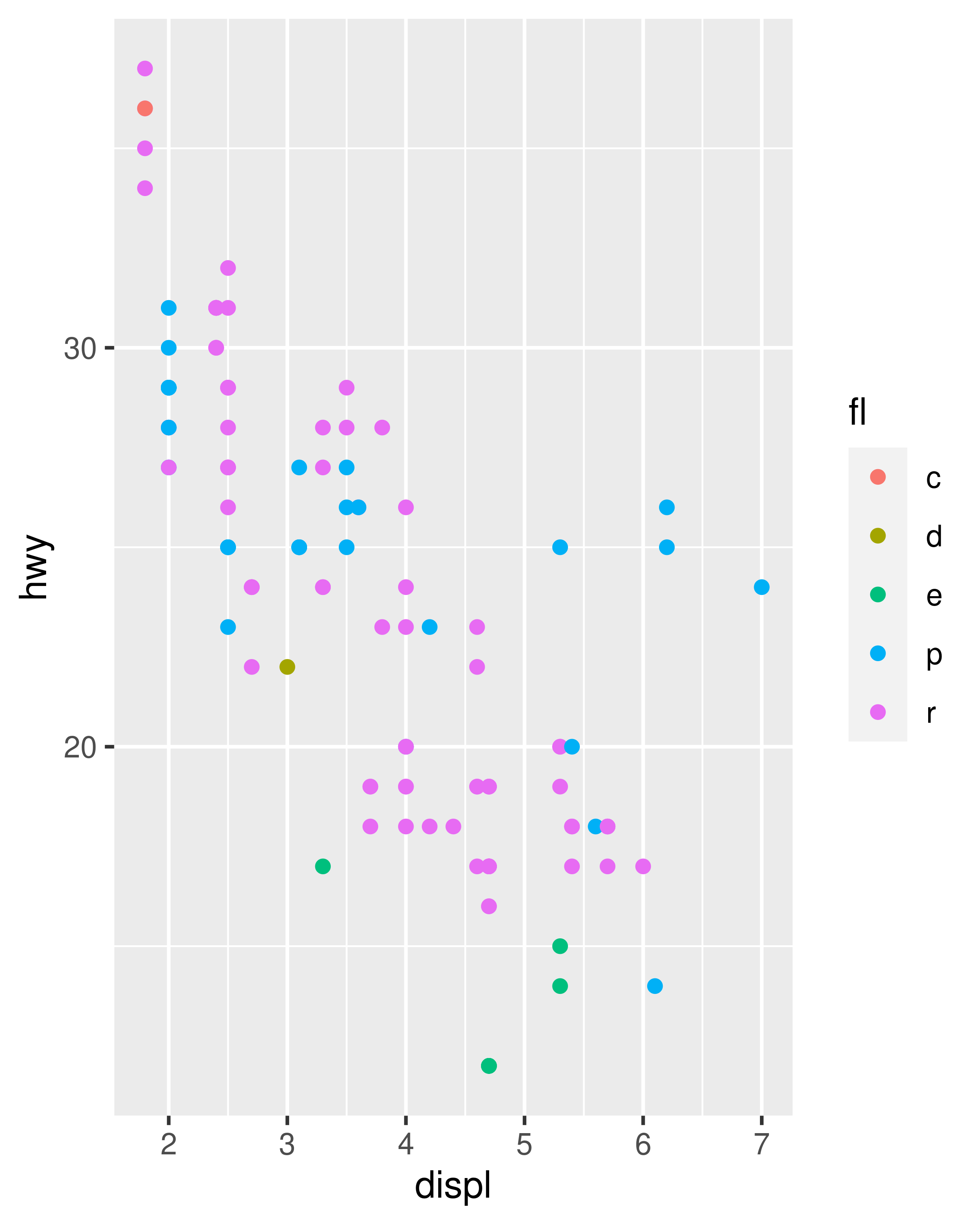
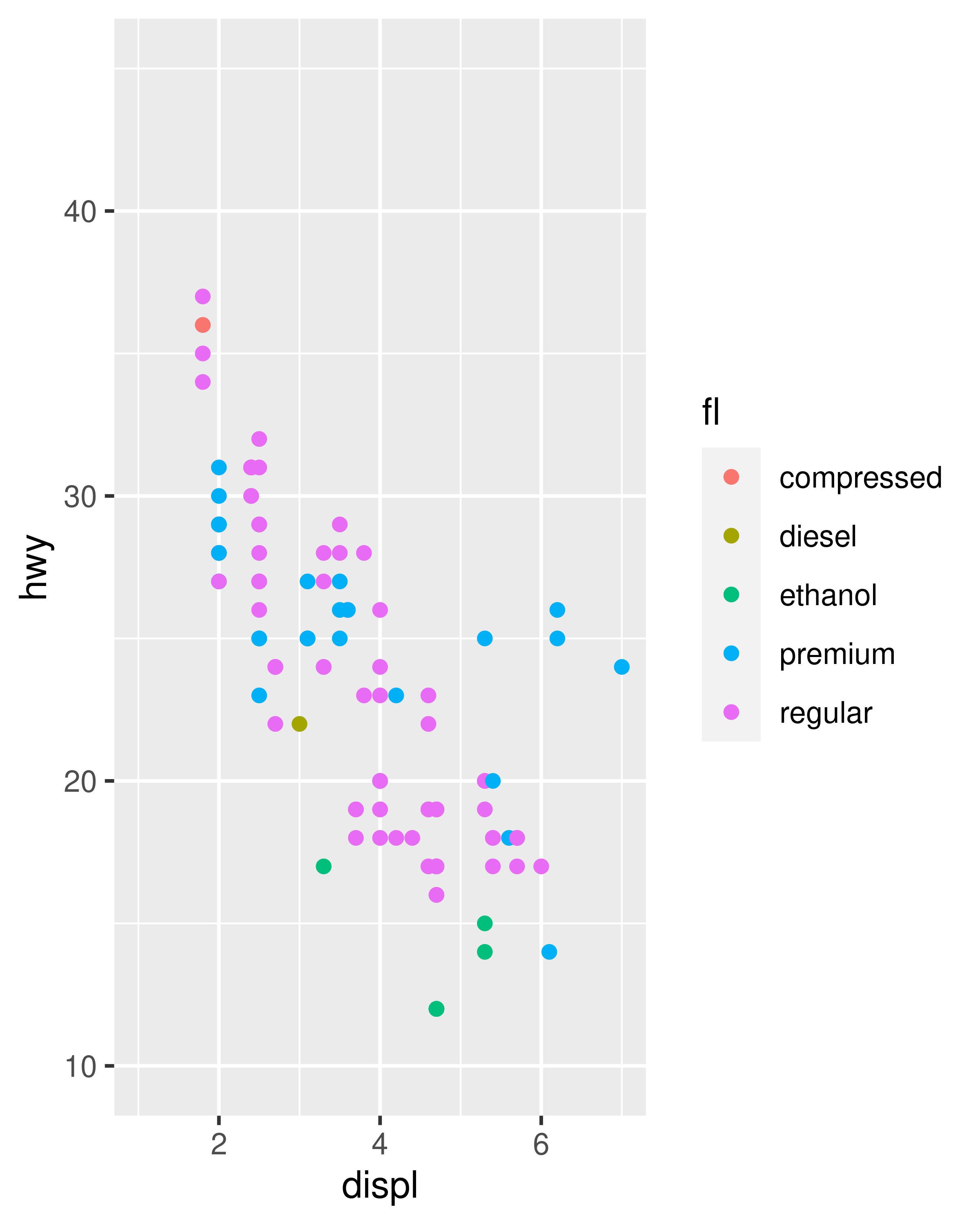
There are two potential limitations to these plots. First, while setting the scale limits does ensure that colours are mapped identically in both plots, it also means that the plot for the 1999 data displays labels for all five fuel types, despite the fact that ethanol and compressed natural gas fuels were not in use at that time. We can address this by manually setting the scale breaks, ensuring that only those fuel types that appear in the data are shown in the legend. The second limitation is that the labels are not particularly helpful, which we can address by specifying them manually. When setting multiple properties of a single scale, it can be more useful to customise using the arguments to the scale function rather than using the lims() helper function:
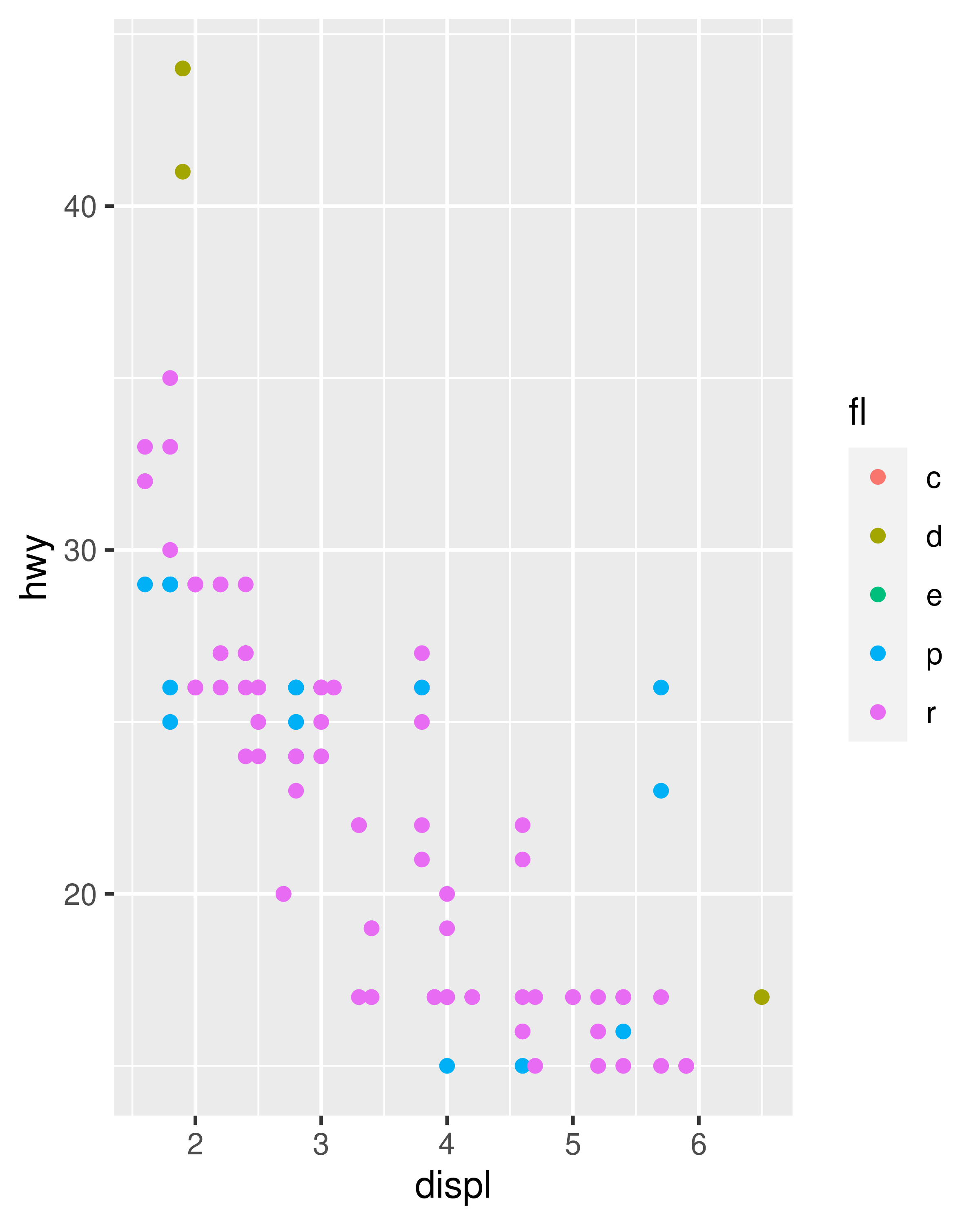
However, there is nothing stopping you from using lims() to control the position aesthetic limits, while using scale_colour_discrete() to exercise more fine-grained control over the colour aesthetic:
base_99 +
  lims(x = c(1, 7), y = c(10, 45)) +
  scale_color_discrete(
    limits = c("c", "d", "e", "p", "r"),
    breaks = c("d", "p", "r"),
    labels = c("diesel", "premium", "regular")
  )

base_08 +
  lims(x = c(1, 7), y = c(10, 45)) +
  scale_color_discrete(
    limits = c("c", "d", "e", "p", "r"),
    labels = c("compressed", "diesel", "ethanol", "premium", "regular")
  )
11.3.6 Legends
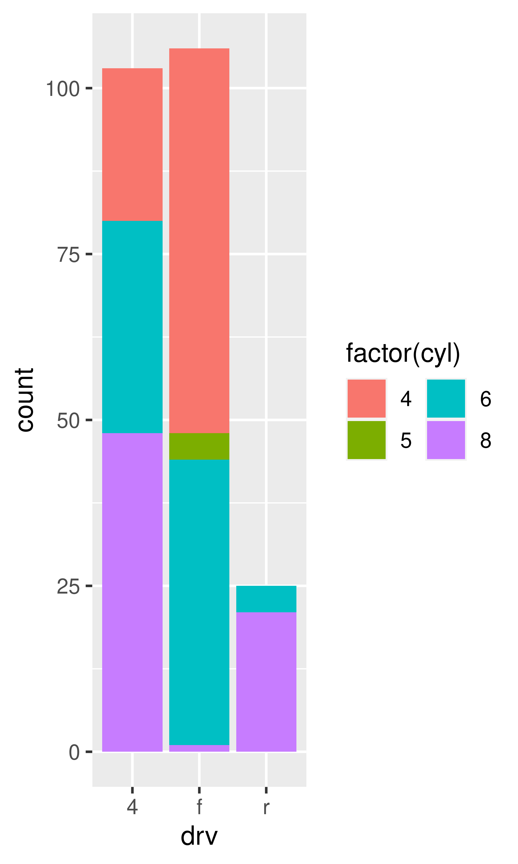
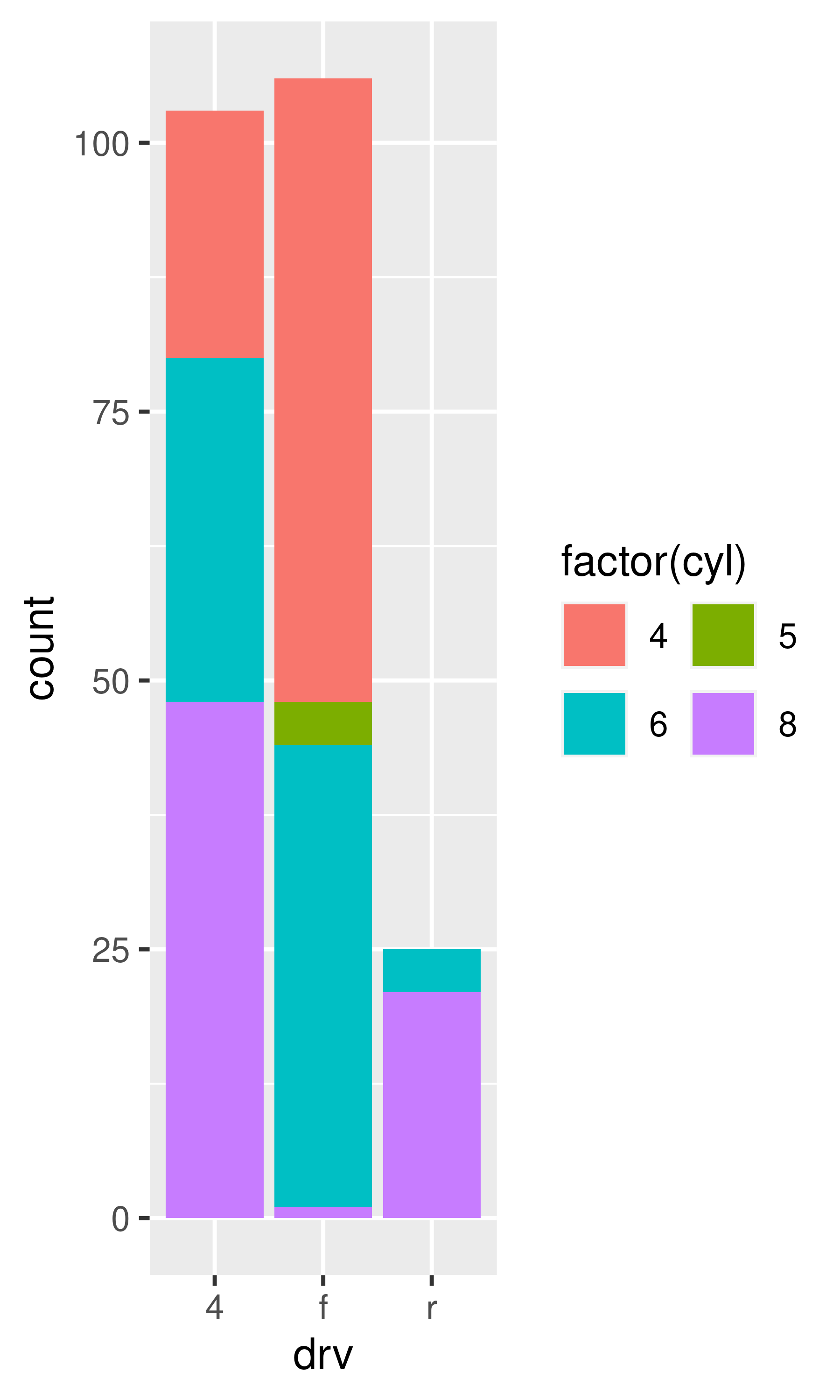
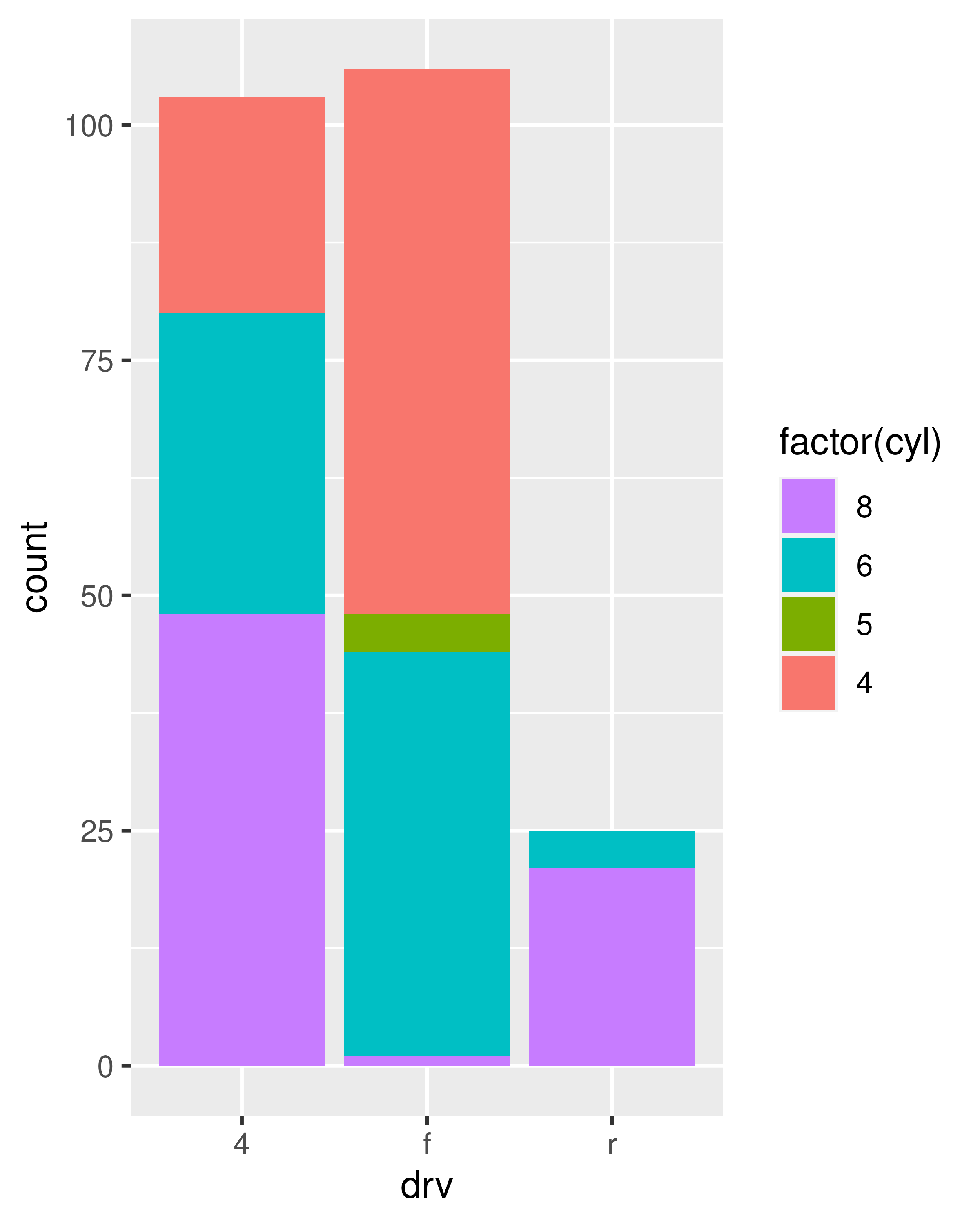
Legends for discrete colour scales can be customised using the guide argument to the scale function or with the guides() helper function, described in Section 11.2.5. For a discrete scale the default legend displays individual keys in a table, which can be customised using guide_legend(). The most useful options are:
-
nroworncolwhich specify the dimensions of the table.byrowcontrols how the table is filled:FALSEfills it by column (the default),TRUEfills it by row.base <- ggplot(mpg, aes(drv, fill = factor(cyl))) + geom_bar() base base + guides(fill = guide_legend(ncol = 2)) base + guides(fill = guide_legend(ncol = 2, byrow = TRUE))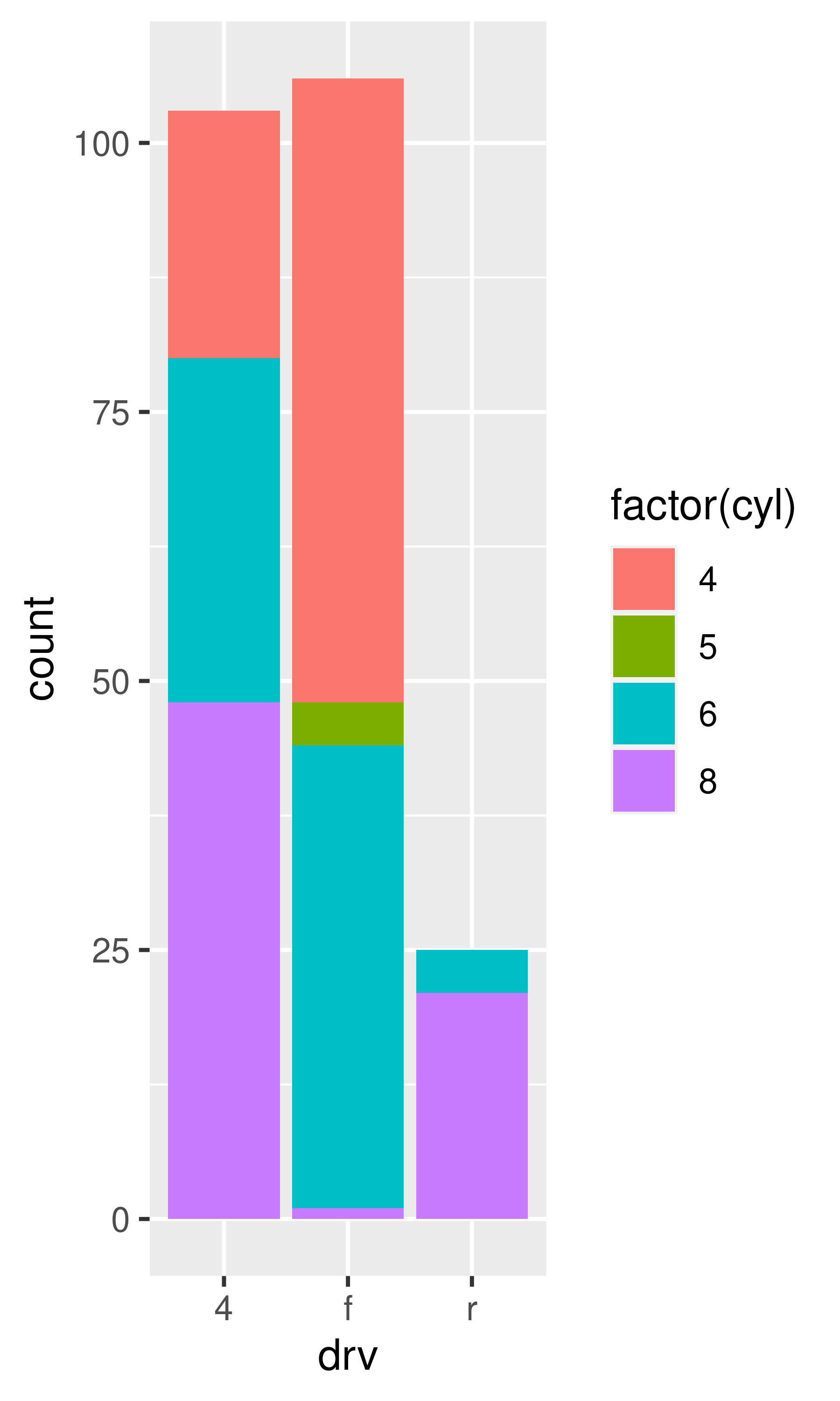
-
reversereverses the order of the keys:base base + guides(fill = guide_legend(reverse = TRUE))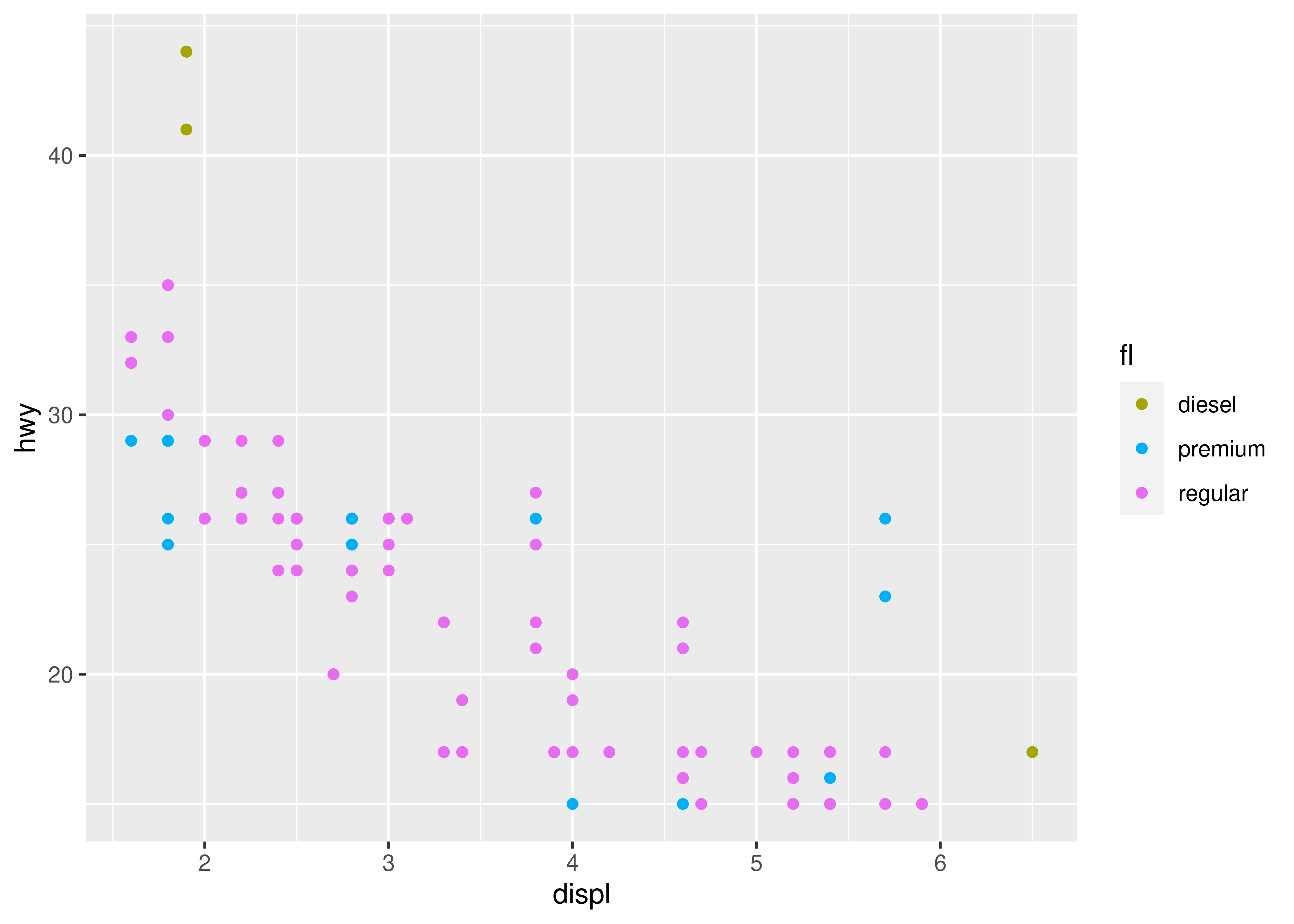

-
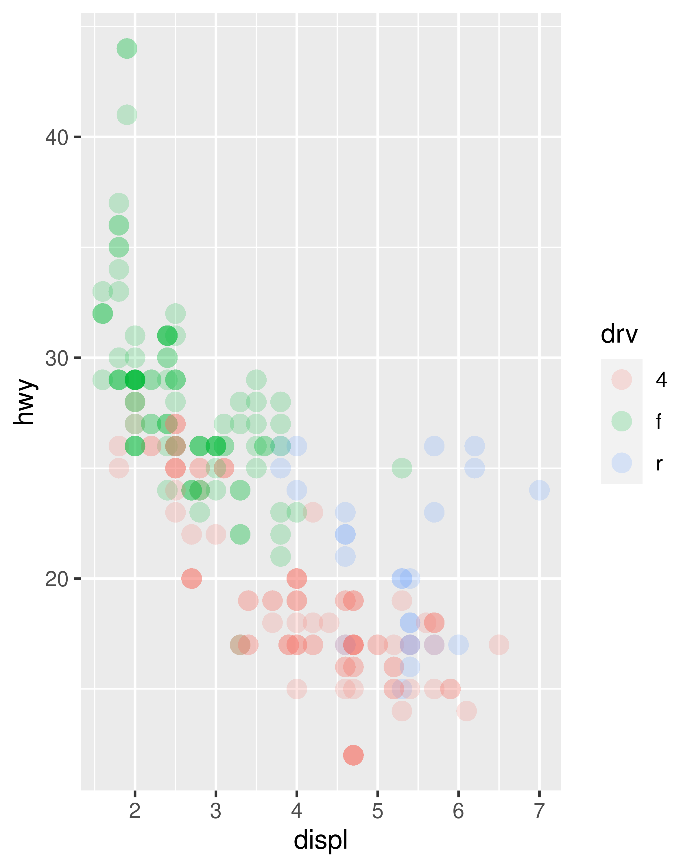
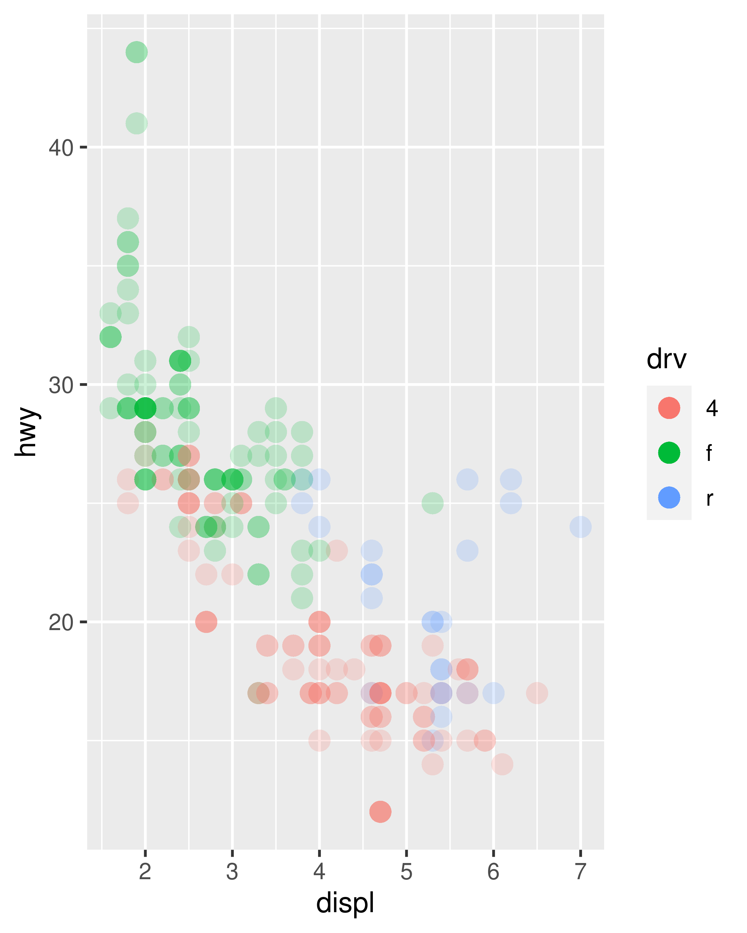
override.aesis useful when you want the elements in the legend display differently to the geoms in the plot. This is often required when you’ve used transparency or size to deal with moderate overplotting and also used colour in the plot.base <- ggplot(mpg, aes(displ, hwy, colour = drv)) + geom_point(size = 4, alpha = .2, stroke = 0) base + guides(colour = guide_legend()) base + guides(colour = guide_legend(override.aes = list(alpha = 1)))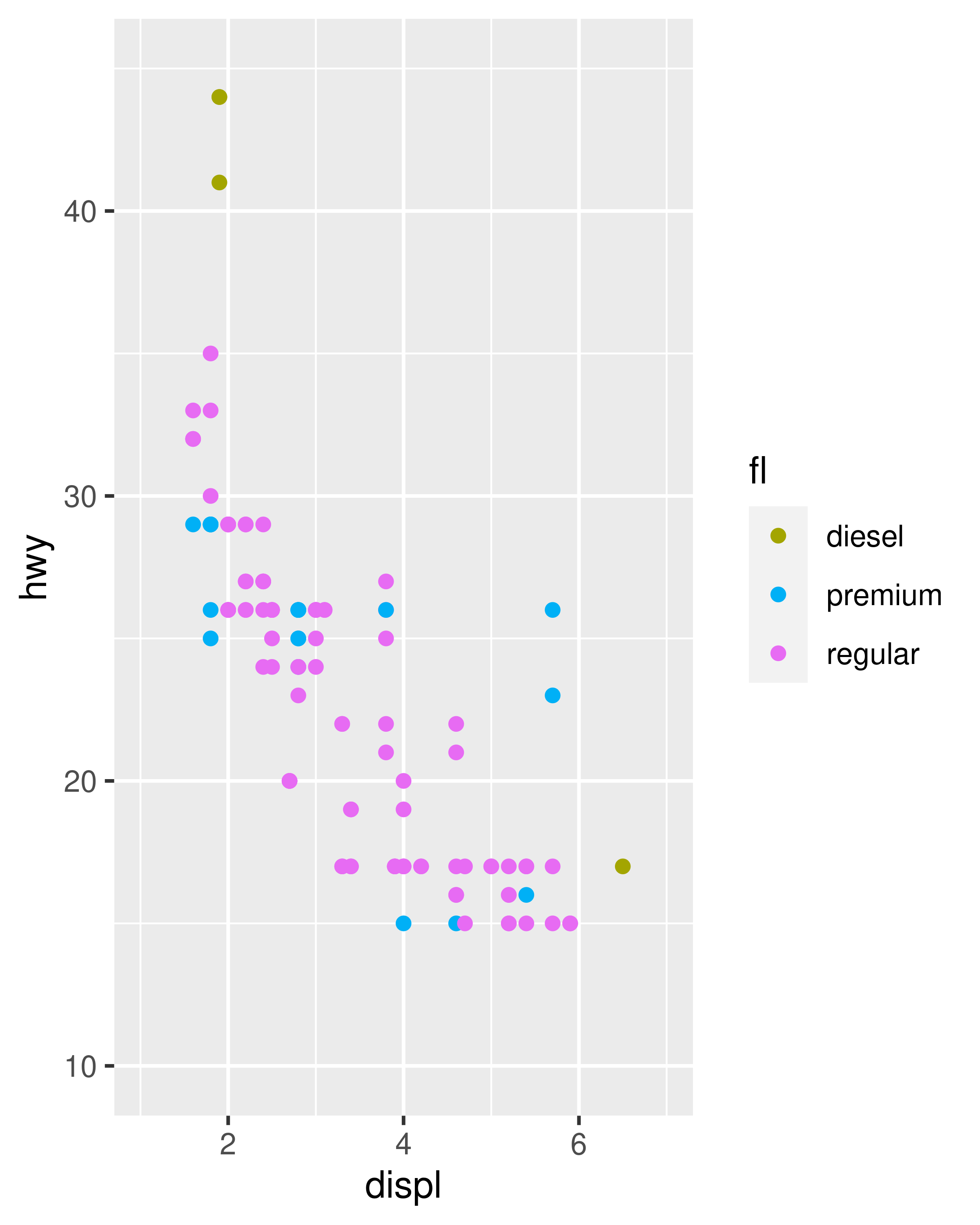
keywidthandkeyheight(along withdefault.unit) allow you to specify the size of the keys. These are grid units, e.g.unit(1, "cm").
You can learn more about guides in Section 14.5.
11.4 Binned colour scales
Colour scales also come in binned versions. The default scale is scale_fill_binned() which in turn defaults to scale_fill_steps(). As with the binned position scales discussed in Section 10.4 these scales have an n.breaks argument that controls the number of discrete colour categories created by the scale. Counterintuitively—because the human visual system is very good at detecting edges—this can sometimes make a continuous colour gradient easier to perceive:
erupt + scale_fill_binned()
erupt + scale_fill_steps()
erupt + scale_fill_steps(n.breaks = 8)


In other respects scale_fill_steps() is analogous to scale_fill_gradient(), and allows you to construct your own two-colour gradients. There is also a three-colour variant scale_fill_steps2() and n-colour scale variant scale_fill_stepsn() that behave similarly to their continuous counterparts:
erupt + scale_fill_steps(low = "grey", high = "brown")
erupt +
  scale_fill_steps2(
    low = "grey",
    mid = "white",
    high = "brown",
    midpoint = .02
  )
erupt + scale_fill_stepsn(n.breaks = 12, colours = terrain.colors(12))

The viridis palettes can be used in the same way, by calling the palette generating functions directly when specifying the colours argument to scale_fill_stepsn():

Alternatively, a brewer analog for binned scales also exists, and is called scale_fill_fermenter():
erupt + scale_fill_fermenter(n.breaks = 9)
erupt + scale_fill_fermenter(n.breaks = 9, palette = "Oranges")
erupt + scale_fill_fermenter(n.breaks = 9, palette = "PuOr")

Note that like the discrete scale_fill_brewer()—and unlike the continuous scale_fill_distiller()—the binned function scale_fill_fermenter() does not interpolate between the brewer colours, and if you set n.breaks larger than the number of colours in the palette a warning message will appear and some colours will not be displayed.
11.4.1 Limits, breaks, and labels
In most respects setting limits, breaks, and labels for a binned scale follows the same logic that applies to continuous scales (Section 10.1.4 and Section 11.2.4). Like a continuous scale, the limits argument is typically a numeric vector of length two specifying the end points, breaks is a numeric vector specifying the break points, and labels is a character vector specifying the labels. All three arguments will accept functions as input (discussed in Section 10.1). The main difference between binned and continuous scales is that the breaks argument defines the edges of the bins rather than simply specifying locations of tick marks.
11.4.2 Legends
The default legend for binned scales uses colour steps rather than a colourbar, and can be customised using the guide_coloursteps() function. A colour step legend shows the area between breaks as a single constant colour, rather than displaying a colour gradient that varies smoothly along the bar. The arguments to guide_coloursteps() mostly mirror those for guide_colourbar() (see Section 11.2.5), with additional arguments that are relevant to binned scales:
-
show.limitsindicates whether values should be shown at the ends of the stepped colour bar, analogous to the corresponding argument inguide_bins()base <- ggplot(mpg, aes(cyl, displ, colour = hwy)) + geom_point(size = 2) + scale_color_binned() base base + guides(colour = guide_coloursteps(show.limits = TRUE))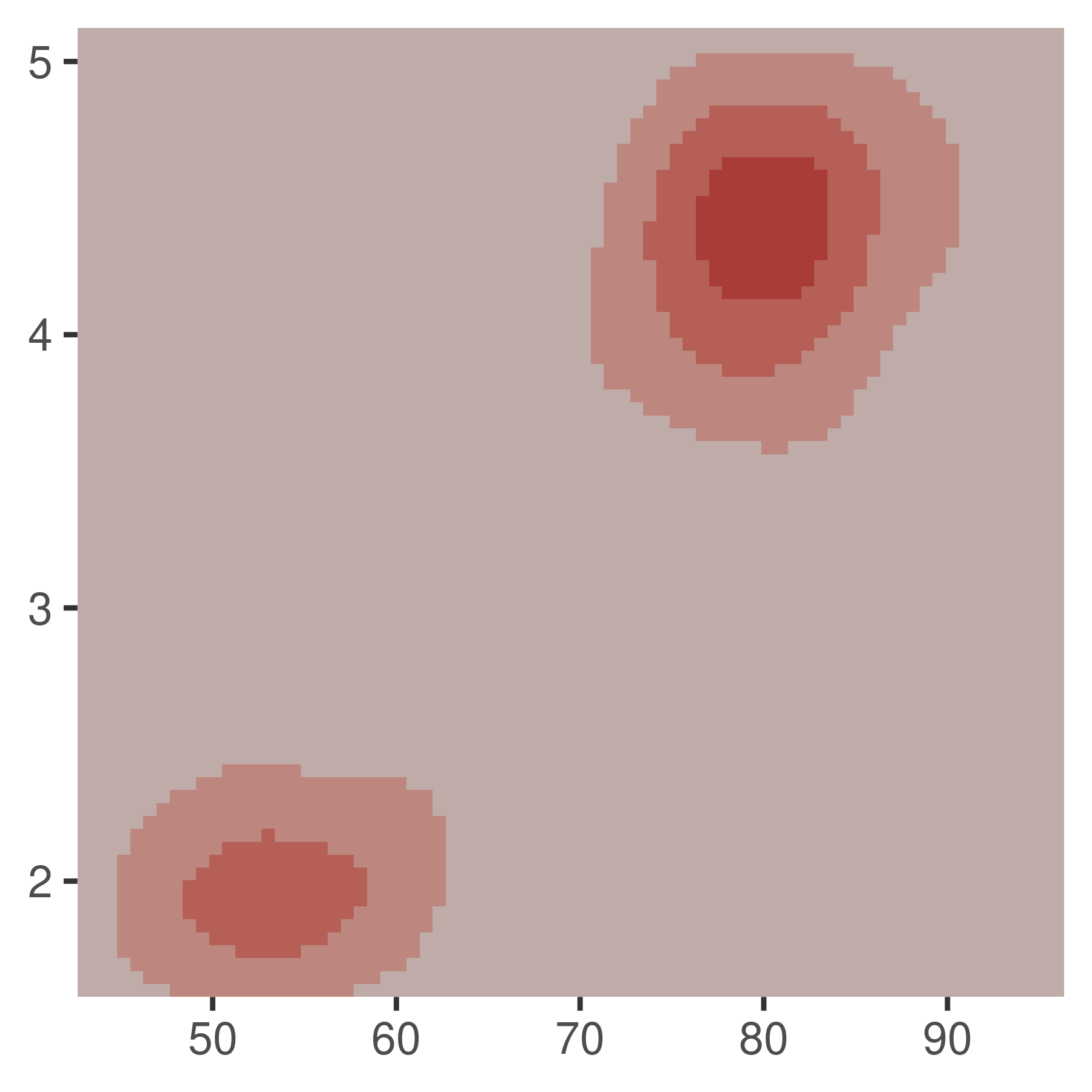
ticksis a logical variable indicating whether tick marks should be displayed adjacent to the legend labels (default isNULL, in which case the value is inherited from the scale)even.stepsis a logical variable indicating whether bins should be evenly spaced (default isTRUE) or proportional in size to their frequency in the data
11.5 Date-time colour scales
When a colour aesthetic is mapped to a date/time type, ggplot2 uses scale_colour_date() or scale_colour_datetime() to specify the scale. These are designed to handle date data, analogous to the date scales discussed in Section 10.2. These scales have date_breaks and date_labels arguments that make it a little easier to work with these data, as the slightly contrived example below illustrates:
base <- ggplot(economics, aes(psavert, uempmed, colour = date)) +
  geom_point()

base
base +
  scale_colour_date(
    date_breaks = "142 months",
    date_labels = "%b %Y"
  )
11.6 Alpha scales
Alpha scales map the transparency of a shade to a value in the data. They are not often useful, but can be a convenient way to visually down-weight less important observations. scale_alpha() is an alias for scale_alpha_continuous() since that is the most common use of alpha, and it saves a bit of typing. An example of an alpha scale using the eruptions data is shown below:
11.7 Legend position
A number of settings that affect the overall display of the legends are controlled through the theme system. You’ll learn more about that in Section 17.2, but for now, all you need to know is that you modify theme settings with the theme() function.
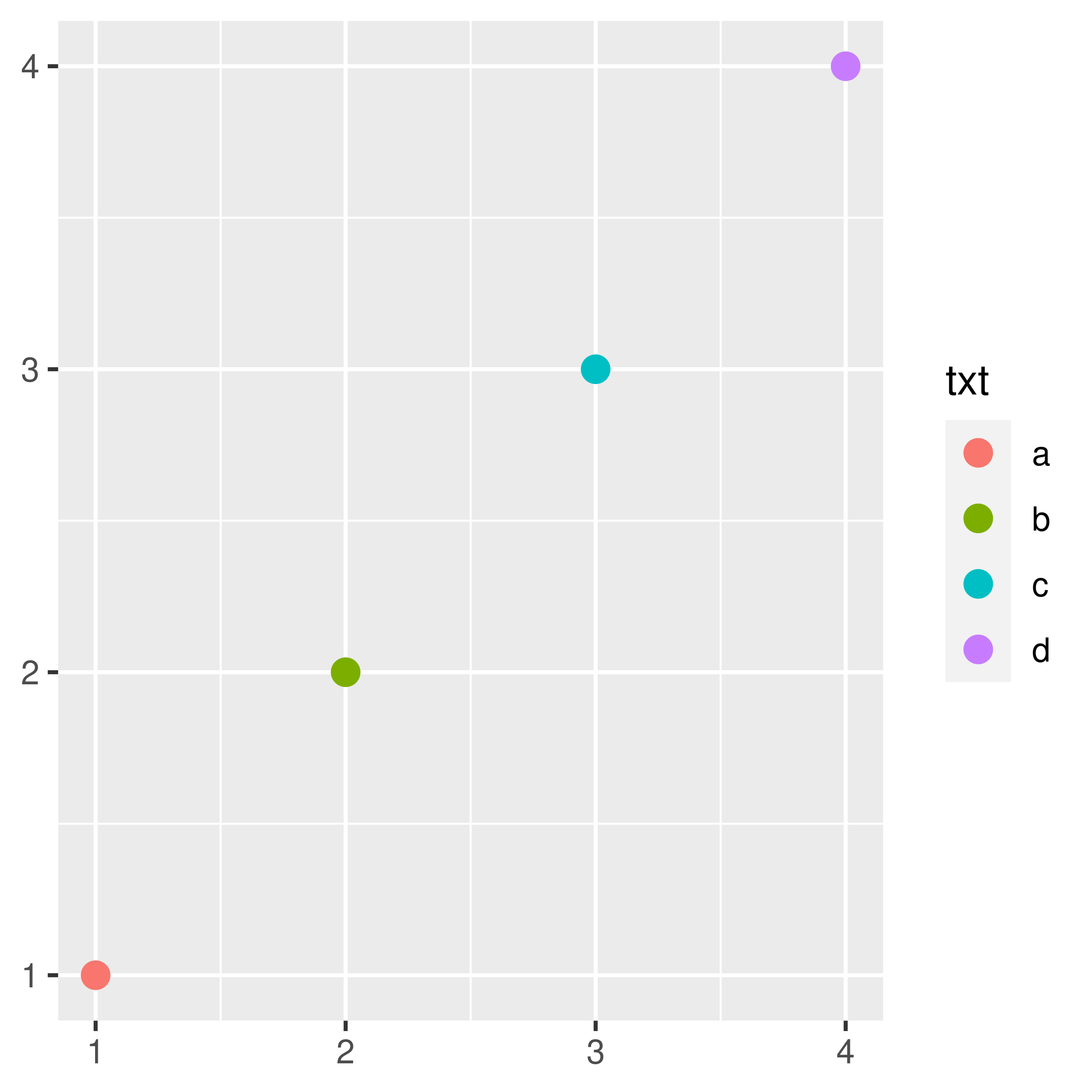
The position and justification of legends are controlled by the theme setting legend.position, which takes values “right”, “left”, “top”, “bottom”, or “none” (no legend).
base <- ggplot(toy, aes(up, up)) +
geom_point(aes(colour = txt), size = 3) +
xlab(NULL) +
ylab(NULL)
base + theme(legend.position = "left")
base + theme(legend.position = "right") # the default
base + theme(legend.position = "bottom")
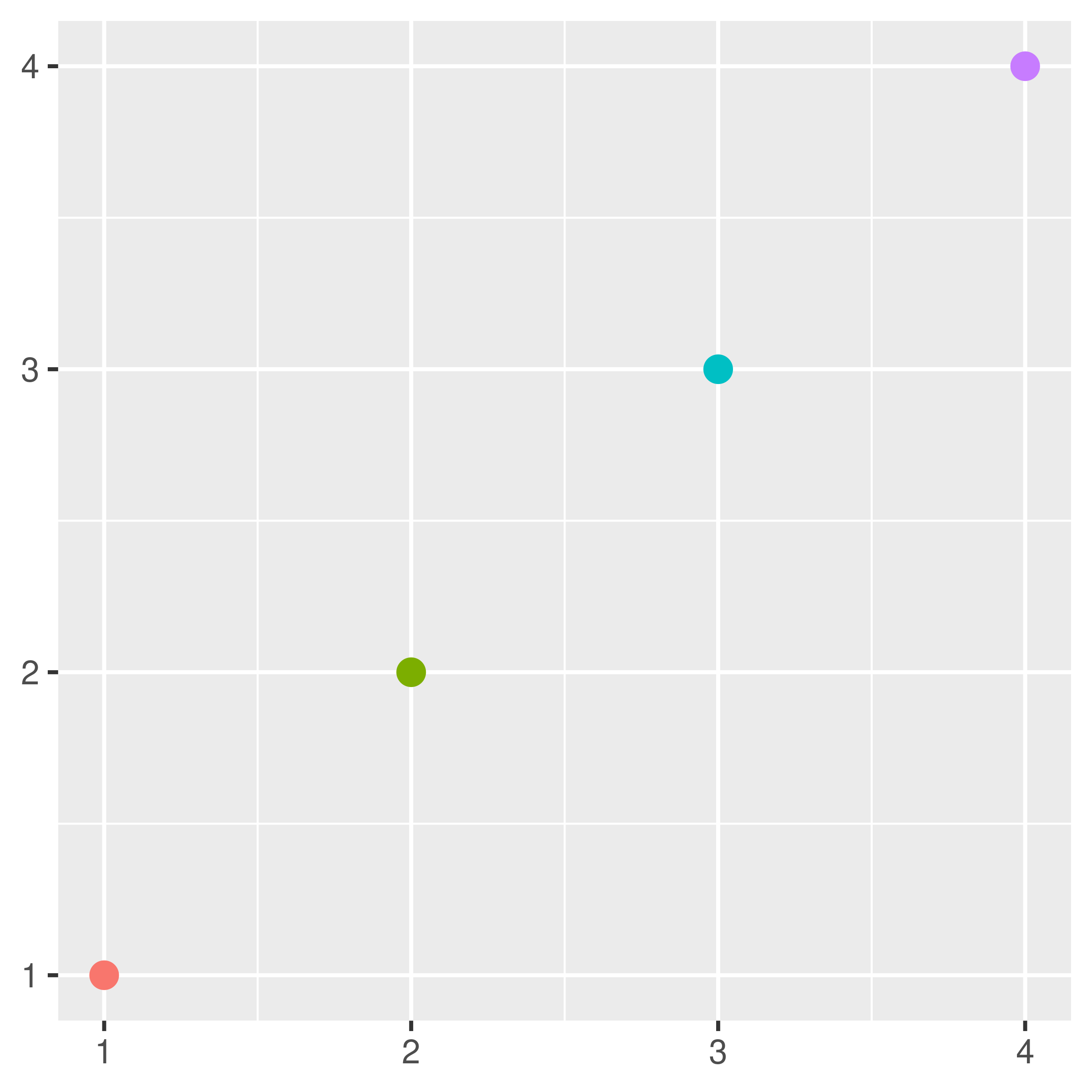
base + theme(legend.position = "none")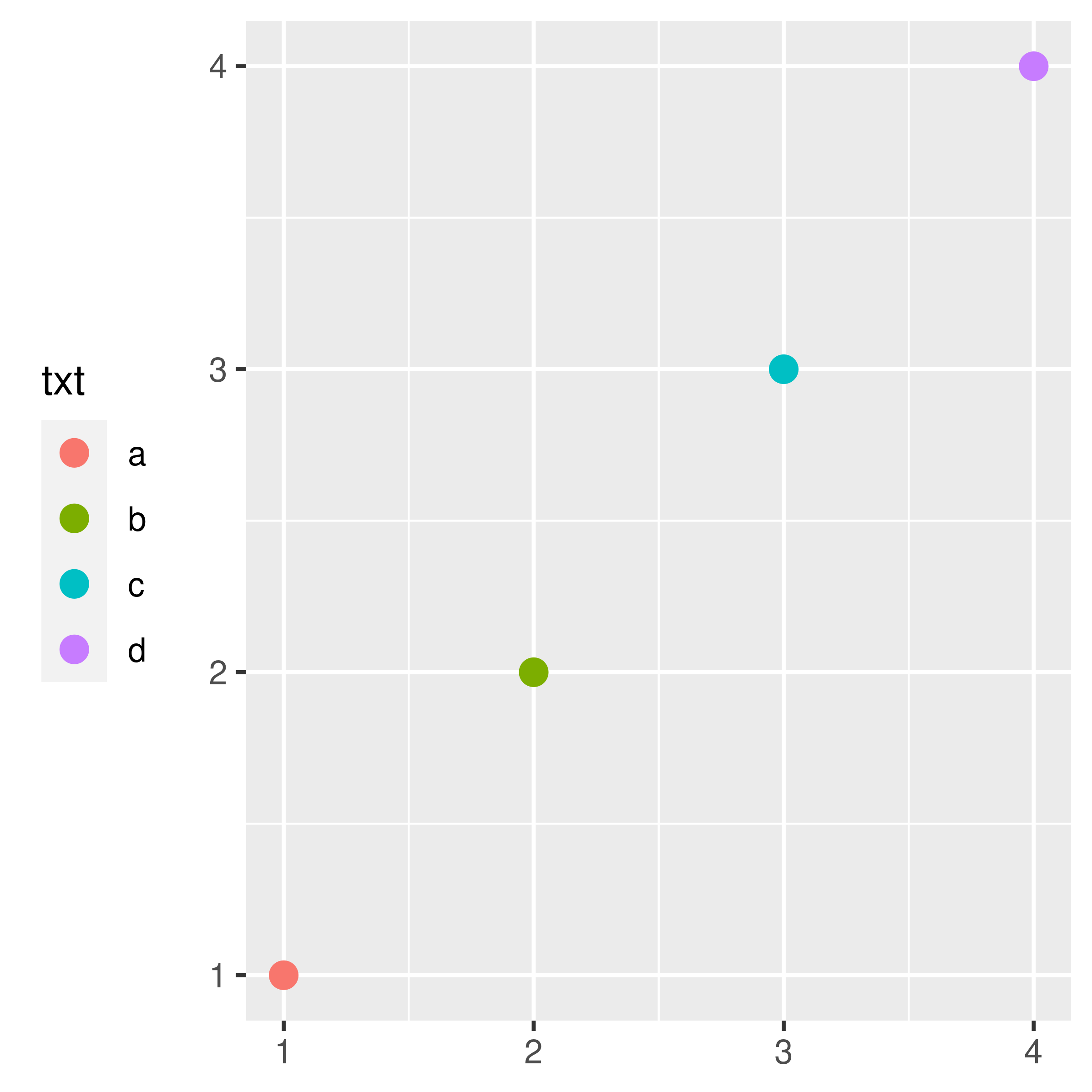
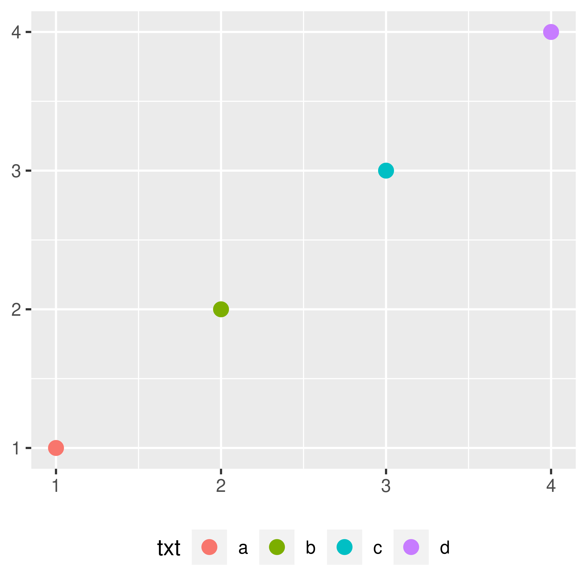
Switching between left/right and top/bottom modifies how the keys in each legend are laid out (horizontal or vertically), and how multiple legends are stacked (horizontal or vertically). If needed, you can adjust those options independently:
legend.direction: layout of items in legends (“horizontal” or “vertical”).legend.box: arrangement of multiple legends (“horizontal” or “vertical”).legend.box.just: justification of each legend within the overall bounding box, when there are multiple legends (“top”, “bottom”, “left”, or “right”).
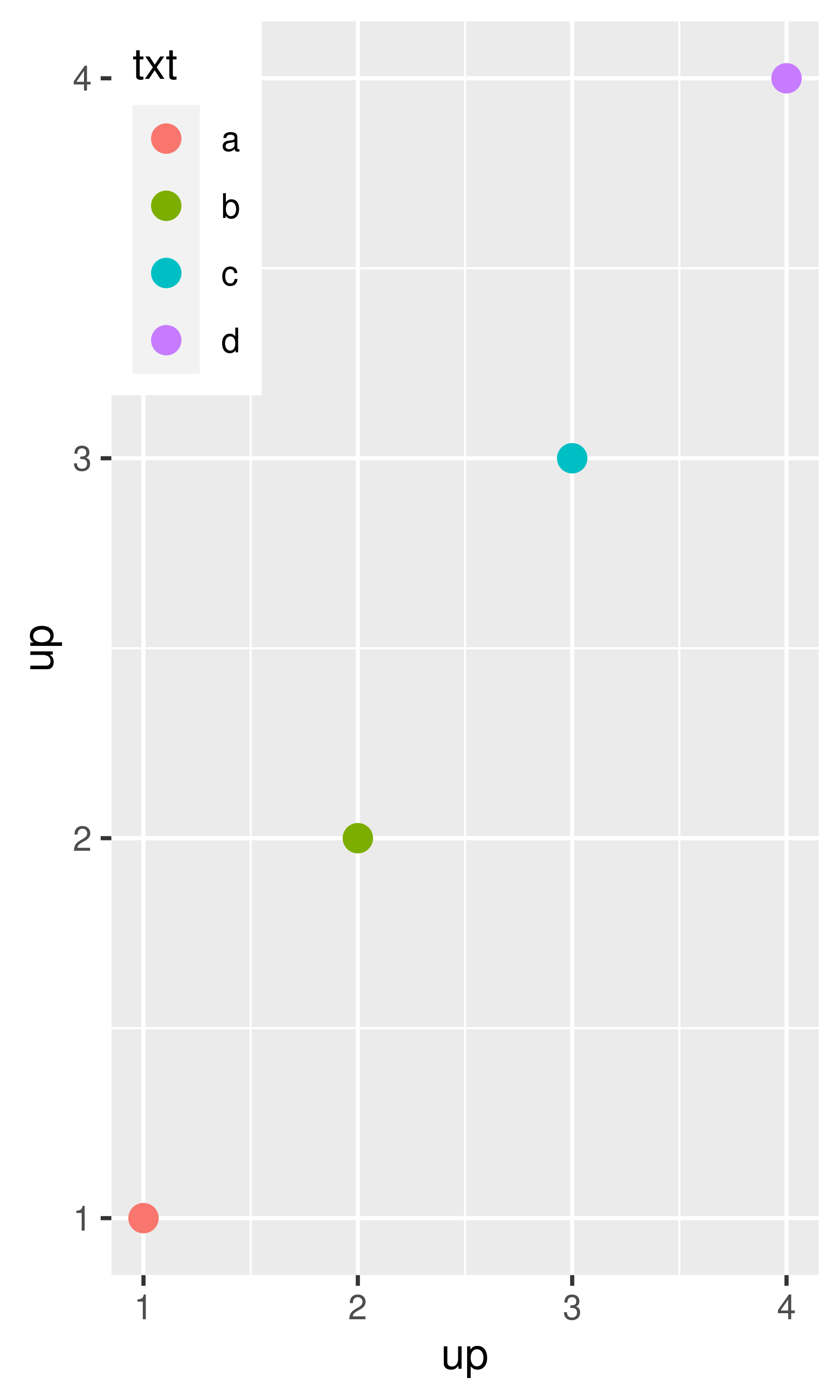
Alternatively, if there’s a lot of blank space in your plot you might want to place the legend inside the plot. You can do this by setting legend.position to a numeric vector of length two. The numbers represent a relative location in the panel area: c(0, 1) is the top-left corner and c(1, 0) is the bottom-right corner. You control which corner of the legend the legend.position refers to with legend.justification, which is specified in a similar way. Unfortunately positioning the legend exactly where you want it requires a lot of trial and error.
base <- ggplot(toy, aes(up, up)) +
geom_point(aes(colour = txt), size = 3)
base +
theme(
legend.position = c(0, 1),
legend.justification = c(0, 1)
)
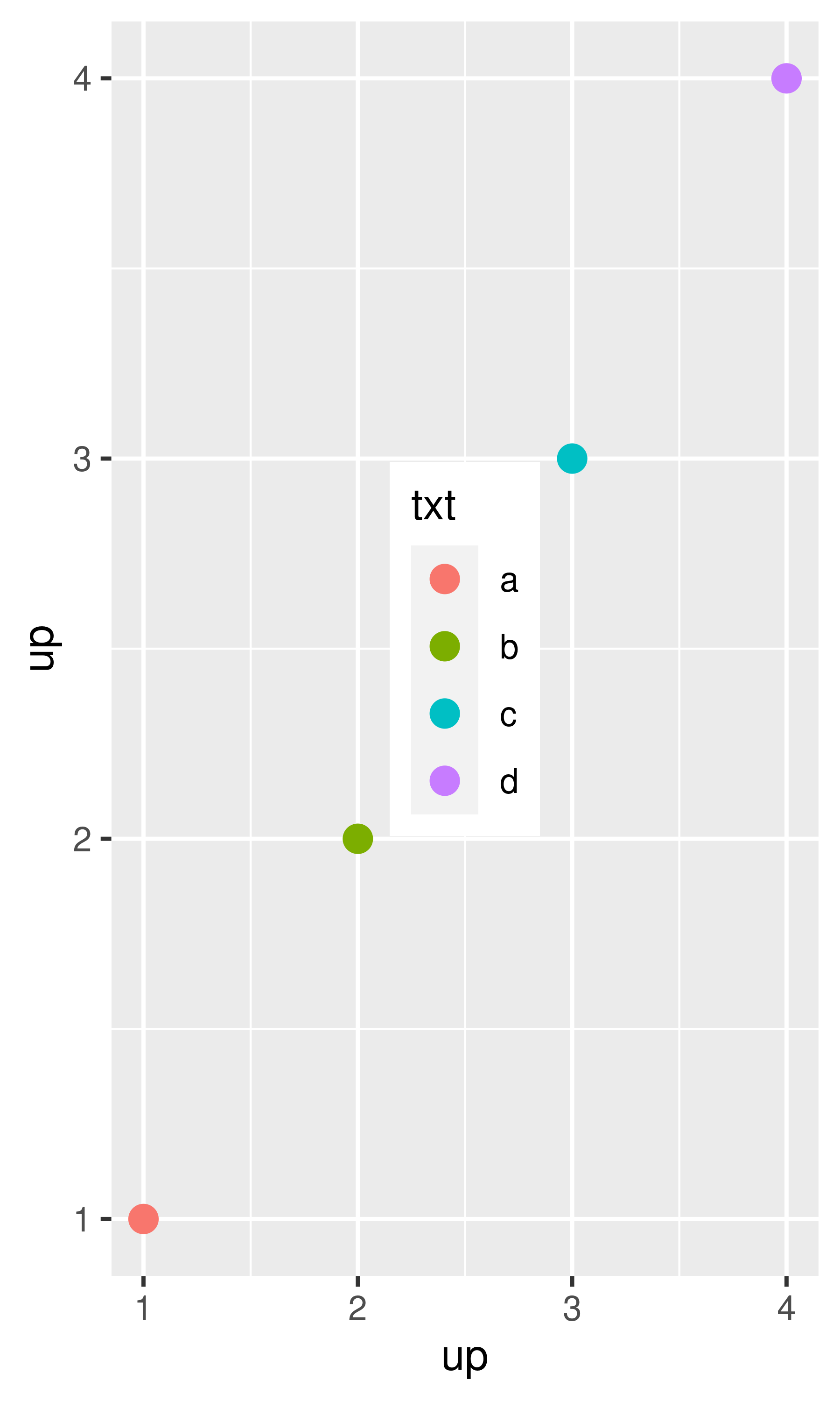
base +
theme(
legend.position = c(0.5, 0.5),
legend.justification = c(0.5, 0.5)
)
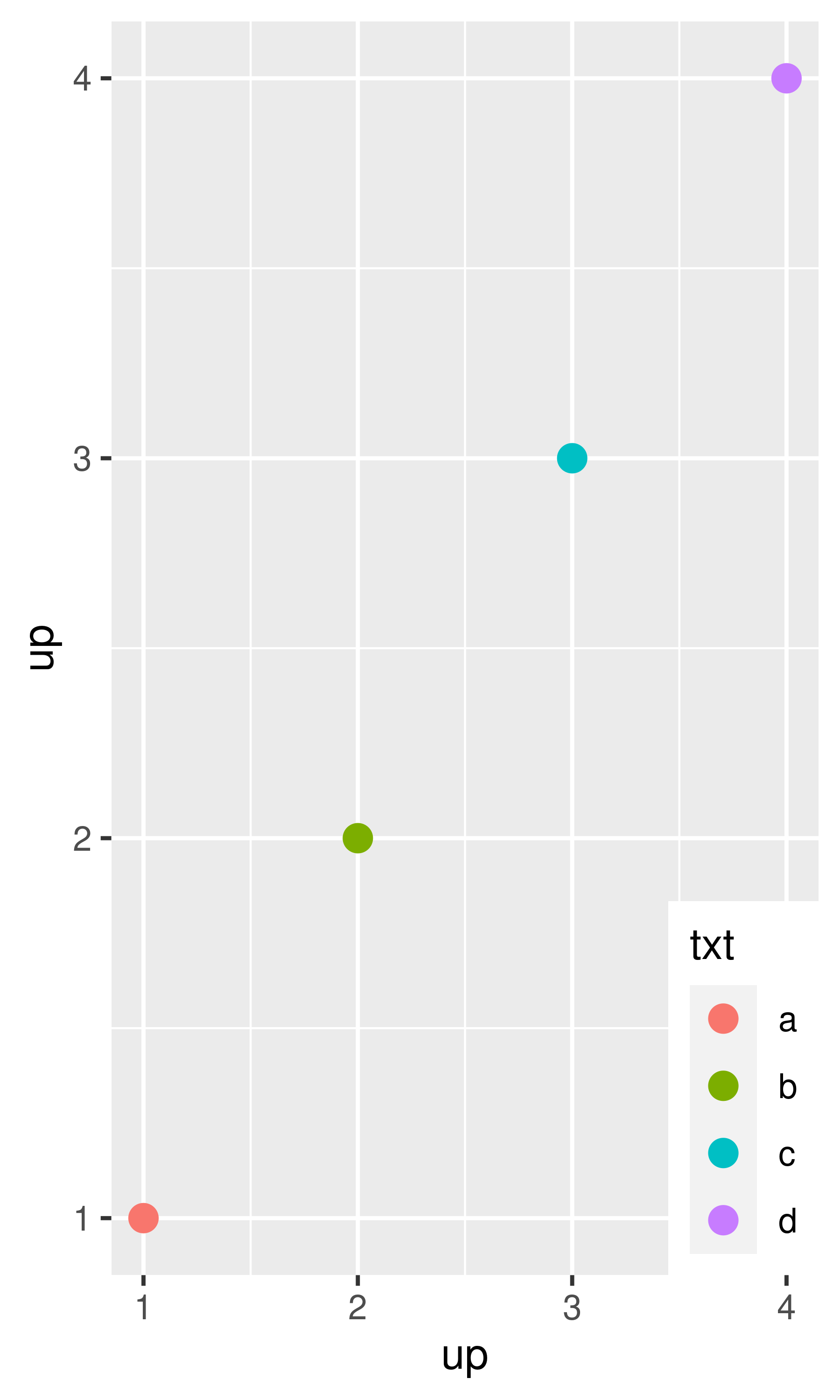
base +
theme(
legend.position = c(1, 0),
legend.justification = c(1, 0)
)
There’s also a margin around the legends, which you can suppress with legend.margin = unit(0, "mm").
Azzalini, A., and A. W. Bowman. 1990. “A Look at Some Data on the Old Faithful Geyser.” Applied Statistics 39: 357–65.
Garnier, Simon. 2018. Viridis: Default Color Maps from ’Matplotlib’. https://CRAN.R-project.org/package=viridis.
Hvitfeldt, Emil. 2020. Paletteer: Comprehensive Collection of Color Palettes. https://CRAN.R-project.org/package=paletteer.
Lumley, Thomas. 2007. Dichromat: Color Schemes for Dichromats.
Ou, Jianhong. 2021. colorBlindness: Safe Color Set for Color Blindness. https://CRAN.R-project.org/package=colorBlindness.
Pedersen, Thomas Lin, and Fabio Crameri. 2020. Scico: Colour Palettes Based on the Scientific Colour-Maps. https://CRAN.R-project.org/package=scico.
Wickham, Charlotte. 2018. Munsell: Utilities for Using Munsell Colours. https://CRAN.R-project.org/package=munsell.
Zeileis, Achim, Kurt Hornik, and Paul Murrell. 2008. “Escaping RGBland: Selecting Colors for Statistical Graphics.” Computational Statistics & Data Analysis. http://statmath.wu-wien.ac.at/~zeileis/papers/Zeileis+Hornik+Murrell-2008.pdf.